24.1.8. Interpolation
24.1.8.1. Heatmap (kernel density estimation)
Creates a density (heatmap) raster of an input point vector layer using kernel density estimation.
The density is calculated based on the number of points in a location, with larger numbers of clustered points resulting in larger values. Heatmaps allow easy identification of hotspots and clustering of points.
Parameters
Label |
Name |
Type |
Description |
|---|---|---|---|
Point layer |
|
[vector: point] |
Point vector layer to use for the heatmap |
Radius |
|
[numeric: double] Default: 100.0 |
Heatmap search radius (or kernel bandwidth) in map units. The radius specifies the distance around a point at which the influence of the point will be felt. Larger values result in greater smoothing, but smaller values may show finer details and variation in point density. |
Output raster size |
|
[numeric: double] Default: 0.1 |
Pixel size of the output raster layer in layer units. In the GUI, the size can be specified by the number of rows
( |
Radius from field Optional |
|
[tablefield: numeric] |
Sets the search radius for each feature from an attribute field in the input layer. |
Weight from field Optional |
|
[tablefield: numeric] |
Allows input features to be weighted by an attribute field. This can be used to increase the influence certain features have on the resultant heatmap. |
Kernel shape |
|
[enumeration] Default: 0 |
Controls the rate at which the influence of a point decreases as the distance from the point increases. Different kernels decay at different rates, so a triweight kernel gives features greater weight for distances closer to the point then the Epanechnikov kernel does. Consequently, triweight results in “sharper” hotspots and Epanechnikov results in “smoother” hotspots. There are many shapes available (please see the Wikipedia page for further information):
|
Decay ratio (Triangular kernels only) Optional |
|
[numeric: double] Default: 0.0 |
Can be used with Triangular kernels to further control how heat from a feature decreases with distance from the feature.
|
Output value scaling |
|
[enumeration] Default: 0 |
Allow to change the values of the output heatmap raster. One of:
|
Heatmap |
|
[raster] Default: |
Specify the output raster layer with kernel density values. One of:
|
Outputs
Label |
Name |
Type |
Description |
|---|---|---|---|
Heatmap |
|
[raster] |
Raster layer with kernel density values |
Example: Creating a Heatmap
For the following example, we will use the airports vector point
layer from the QGIS sample dataset (see Downloading sample data).
Another excellent QGIS tutorial on making heatmaps can be found at
http://qgistutorials.com.
In Fig. 24.24, the airports of Alaska are shown.
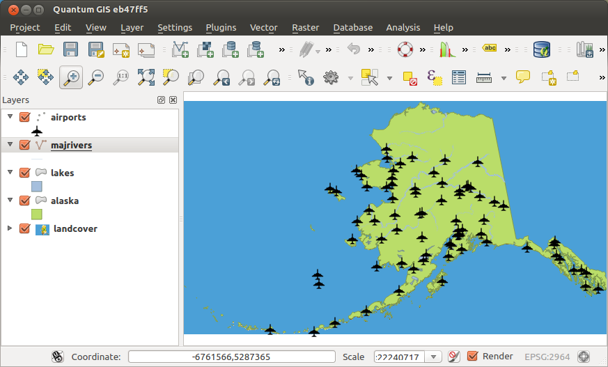
Fig. 24.24 Airports of Alaska
Open the Heatmap (Kernel Density Estimation) algorithm from the QGIS Interpolation group
In the Point layer
 field, select
airportsfrom the list of point layers loaded in the current project.Change the Radius to
1000000meters.Change the Pixel size X to
1000. The Pixel size Y, Rows and Columns will be automatically updated.Click on Run to create and load the airports heatmap (see Fig. 24.26).
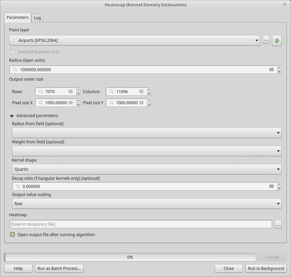
Fig. 24.25 The Heatmap Dialog
QGIS will generate the heatmap and add it to your map window. By default, the heatmap is shaded in greyscale, with lighter areas showing higher concentrations of airports. The heatmap can now be styled in QGIS to improve its appearance.
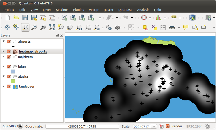
Fig. 24.26 The heatmap after loading looks like a grey surface
Open the properties dialog of the
heatmap_airportslayer (select the layerheatmap_airports, open the context menu with the right mouse button and select Properties).Select the Symbology tab.
Change the Render type
to
‘Singleband pseudocolor’.Select a suitable Color ramp
, for
instance YlOrRd.Click the Classify button.
Press OK to update the layer.
The final result is shown in Fig. 24.27.
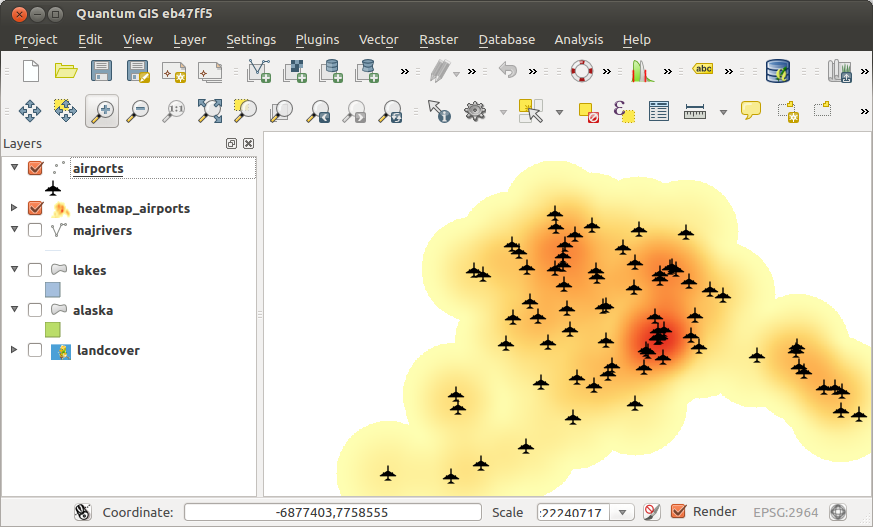
Fig. 24.27 Styled heatmap of airports of Alaska
Python code
Algorithm ID: qgis:heatmapkerneldensityestimation
import processing
processing.run("algorithm_id", {parameter_dictionary})
The algorithm id is displayed when you hover over the algorithm in the Processing Toolbox. The parameter dictionary provides the parameter NAMEs and values. See Using processing algorithms from the console for details on how to run processing algorithms from the Python console.
24.1.8.2. IDW Interpolation
Generates an Inverse Distance Weighted (IDW) interpolation of a point vector layer.
Sample points are weighted during interpolation such that the influence of one point relative to another declines with distance from the unknown point you want to create.
The IDW interpolation method also has some disadvantages: the quality of the interpolation result can decrease, if the distribution of sample data points is uneven.
Furthermore, maximum and minimum values in the interpolated surface can only occur at sample data points.
Parameters
Label |
Name |
Type |
Description |
|---|---|---|---|
Input layer(s) |
|
[string] |
Vector layer(s) and field(s) to use for the interpolation,
coded in a string (see the The following GUI elements are provided to compose the interpolation data string:
For each of the added layer-field combinations, a type can be chosen:
In the string, the layer-field elements are separated by
|
Distance coefficient P |
|
[numeric: double] Default: 2.0 |
Sets the distance coefficient for the interpolation. Minimum: 0.0, maximum: 100.0. |
Extent (xmin, xmax, ymin, ymax) |
|
[extent] |
Extent of the output raster layer. Available methods are:
|
Output raster size |
|
[numeric: double] Default: 0.1 |
Pixel size of the output raster layer in layer units. In the GUI, the size can be specified by the number of rows
( |
Interpolated |
|
[raster] Default: |
Raster layer of interpolated values. One of:
|
Outputs
Label |
Name |
Type |
Description |
|---|---|---|---|
Interpolated |
|
[raster] |
Raster layer of interpolated values |
Python code
Algorithm ID: qgis:idwinterpolation
import processing
processing.run("algorithm_id", {parameter_dictionary})
The algorithm id is displayed when you hover over the algorithm in the Processing Toolbox. The parameter dictionary provides the parameter NAMEs and values. See Using processing algorithms from the console for details on how to run processing algorithms from the Python console.
24.1.8.3. Line Density
Calculates for each raster cell, the density measure of linear features within a circular neighbourhood. This measure is obtained by summing all the line segments intersecting the circular neighbourhood and dividing this sum by the area of such neighbourhood. A weighting factor can be applied to the line segments.
Note
This algorithm uses ellipsoid based measurements and respects the current ellipsoid settings.
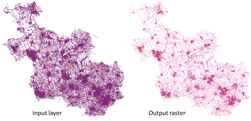
Fig. 24.28 Line density example. Input layer source: Roads Overijssel - The Netherlands (OSM).
Parameters
Basic parameters
Label |
Name |
Type |
Description |
|---|---|---|---|
Input line layer |
|
[vector: line] |
Input vector layer containing line features |
Weight field |
|
[tablefield: numeric] |
Field of the layer containing the weight factor to use during the calculation |
Search Radius |
|
[numeric: double] Default: 10.0 |
Radius of the circular neighbourhood. Units can be specified here. |
Pixel size |
|
[numeric: double] Default: 10.0 |
Pixel size of the output raster layer in layer units. The raster has square pixels. |
Line density raster |
|
[raster] Default: |
The output as a raster layer. One of:
|
Advanced parameters
Label |
Name |
Type |
Description |
|---|---|---|---|
Creation options Optional
|
|
[string] Default: ‘’ |
For adding one or more creation options that control the raster to be created (colors, block size, file compression…). For convenience, you can rely on predefined profiles (see GDAL driver options section). Batch Process and Model Designer: separate multiple options with a pipe
character ( |
Outputs
Label |
Name |
Type |
Description |
|---|---|---|---|
Line density raster |
|
[raster] |
The output line density raster layer. |
Python code
Algorithm ID: native:linedensity
import processing
processing.run("algorithm_id", {parameter_dictionary})
The algorithm id is displayed when you hover over the algorithm in the Processing Toolbox. The parameter dictionary provides the parameter NAMEs and values. See Using processing algorithms from the console for details on how to run processing algorithms from the Python console.
24.1.8.4. TIN Interpolation
Generates a Triangulated Irregular Network (TIN) interpolation of a point vector layer.
With the TIN method you can create a surface formed by triangles of nearest neighbor points. To do this, circumcircles around selected sample points are created and their intersections are connected to a network of non overlapping and as compact as possible triangles. The resulting surfaces are not smooth.
The algorithm creates both the raster layer of the interpolated values and the vector line layer with the triangulation boundaries.
Parameters
Label |
Name |
Type |
Description |
|---|---|---|---|
Input layer(s) |
|
[string] |
Vector layer(s) and field(s) to use for the interpolation,
coded in a string (see the The following GUI elements are provided to compose the interpolation data string:
For each of the added layer-field combinations, a type can be chosen:
In the string, the layer-field elements are separated by
|
Interpolation method |
|
[enumeration] Default: 0 |
Set the interpolation method to be used. One of:
|
Extent (xmin, xmax, ymin, ymax) |
|
[extent] |
Extent of the output raster layer. Available methods are:
|
Output raster size |
|
[numeric: double] Default: 0.1 |
Pixel size of the output raster layer in layer units. In the GUI, the size can be specified by the number of rows
( |
Interpolated |
|
[raster] Default: |
The output TIN interpolation as a raster layer. One of:
|
Triangulation |
|
[vector: line] Default: |
The output TIN as a vector layer. One of:
The file encoding can also be changed here. |
Outputs
Label |
Name |
Type |
Description |
|---|---|---|---|
Interpolated |
|
[raster] |
The output TIN interpolation as a raster layer |
Triangulation |
|
[vector: line] |
The output TIN as a vector layer. |
Python code
Algorithm ID: qgis:tininterpolation
import processing
processing.run("algorithm_id", {parameter_dictionary})
The algorithm id is displayed when you hover over the algorithm in the Processing Toolbox. The parameter dictionary provides the parameter NAMEs and values. See Using processing algorithms from the console for details on how to run processing algorithms from the Python console.