7. QGIS GUI
Die grafische Benutzeroberfläche (GUI) von QGIS ist in der unteren Abbildung dargestellt (die Zahlen 1 bis 5 in den gelben Kreisen kennzeichnen wichtige Elemente der Oberfläche und werden nachfolgend erläutert).
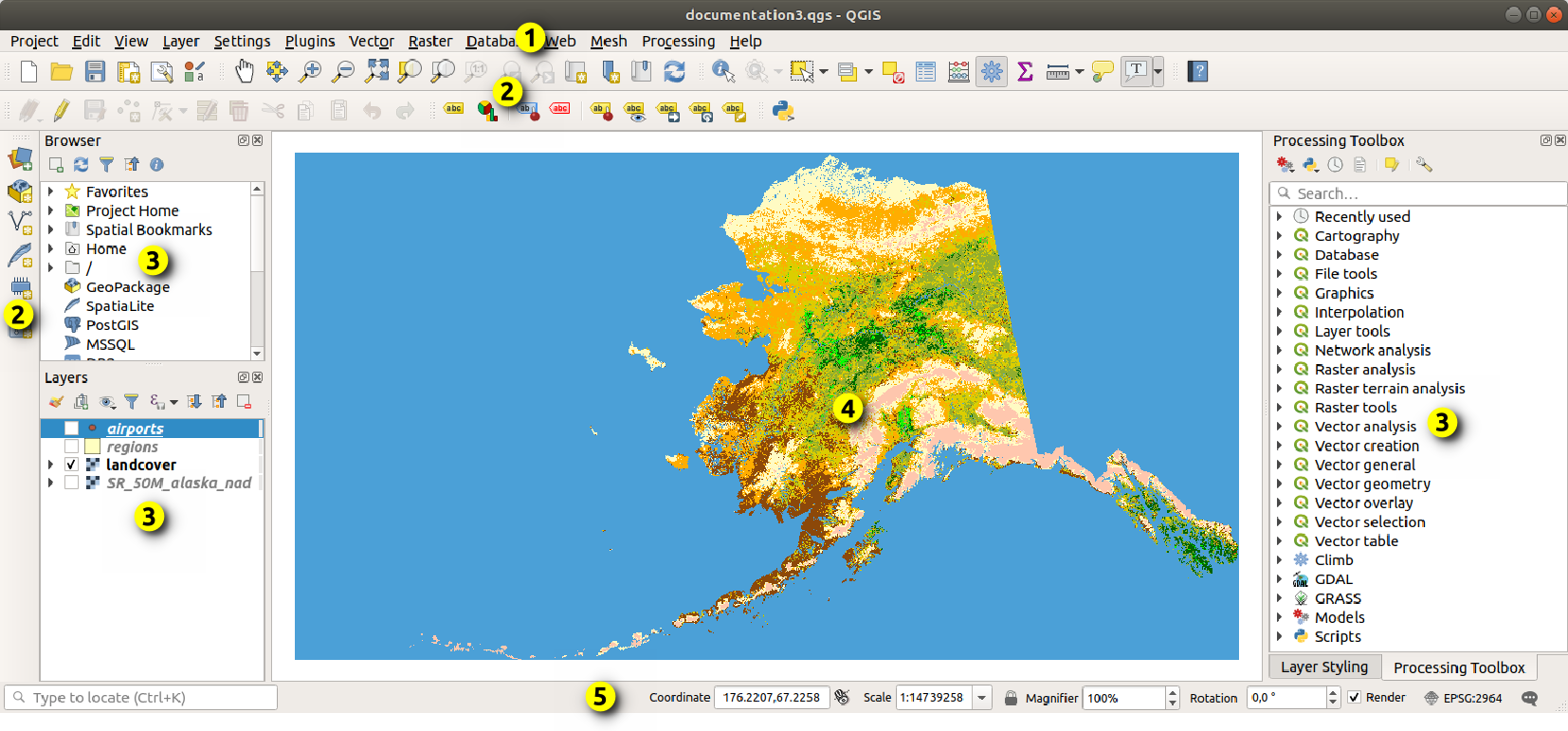
Abb. 7.1 QGIS GUI mit Alaskabeispieldatensatz
Bemerkung
Das Aussehen einzelner Bereiche (Titelleiste, etc.) kann in Abhängigkeit vom Betriebssystem und dem Fenstermanager abweichen.
Das QGIS-Hauptfenster (Abb. 7.1) setzt sich aus fünf Bestandteilen bzw. Arten von Bestandteilen zusammen:
Scroll down for detailed explanations of these.
7.1. Menüleiste
The Menu bar provides access to QGIS functions using standard hierarchical menus. The Menus, their options, associated icons and keyboard shortcuts are described below. The keyboard shortcuts can be reconfigured ().
Most menu options have a corresponding tool and vice-versa. However, the Menus are not organized exactly like the toolbars. The locations of menu options in the toolbars are indicated below in the table. Plugins may add new options to Menus. For more information about tools and toolbars, see Werkzeugkästen.
Bemerkung
QGIS is a cross-platform application. Tools are generally available on all platforms, but they may be placed in different menus, depending on the operating systems. The lists below show the most common locations, including known variations.
7.1.1. Projekt
The menu provides access and exit points for project files. It provides tools to:
Create a New project file from scratch or use another project file as a template (see Project files options for template configuration)
Open… a project from a file, a GeoPackage or a PostgreSQL database
Close a project or revert it to its last saved state
Save a project in
.qgsor.qgzfile format, either as a file or within a GeoPackage or PostgreSQL databaseExport the map canvas to different formats or use a print layout for more complex output
Set project properties and snapping options for geometry editing.
Menüleiste |
Tastenkürzel |
Werkzeugleiste |
Referenz |
|---|---|---|---|
|
Ctrl+N |
Projekt |
|
|
Strg+O |
Projekt |
|
Alt+J + R |
|||
Schließen |
|||
|
Strg+S |
Projekt |
|
|
Strg+Shift+S |
Projekt |
|
Revert… |
|||
|
Strg+Shift+P |
||
Fangoptionen… |
|||
|
|||
|
|||
|
Strg+P |
Projekt |
|
|
|||
|
Projekt |
||
|
Strg+Q |


Under  macOS, the Exit QGIS command corresponds to
(Cmd+Q).
macOS, the Exit QGIS command corresponds to
(Cmd+Q).
7.1.2. Bearbeiten
The menu provides most of the native tools needed to edit layer attributes or geometry (see Editierfunktionen for details).
Menüleiste |
Tastenkürzel |
Werkzeugleiste |
Referenz |
|---|---|---|---|
|
Strg+Z |
Digitalisierung |
|
|
Strg+Shift+Z |
Digitalisierung |
|
|
Strg+X |
Digitalisierung |
|
|
Strg+C |
Digitalisierung |
|
|
Strg+V |
Digitalisierung |
|
Ctrl+Alt+V |
|||
|
Digitalisierung |
||
|
Selection |
||
|
Selection |
||
|
Selection |
||
|
Selection |
||
|
F3 |
Selection |
|
|
Ctrl+F3 |
Selection |
|
|
Ctrl+Alt+A |
Selection |
|
|
Strg+Umschalt+A |
Selection |
|
|
Strg+A |
Selection |
|
|
Selection |
||
|
Strg+. |
Digitalisierung |
|
|
Strg+. |
Digitalisierung |
|
|
Strg+. |
Digitalisierung |
|
|
Strg+. |
Digitalisierung |
|
|
Shape Digitizing |
||
|
Shape Digitizing |
||
Shape Digitizing |
|||
|
Shape Digitizing |
||
|
Shape Digitizing |
||
|
Shape Digitizing |
||
|
Shape Digitizing |
||
|
Shape Digitizing |
||
Shape Digitizing |
|||
|
Shape Digitizing |
||
|
Shape Digitizing |
||
|
Shape Digitizing |
||
|
Shape Digitizing |
||
Shape Digitizing |
|||
|
Shape Digitizing |
||
|
Shape Digitizing |
||
|
Shape Digitizing |
||
Shape Digitizing |
|||
|
Shape Digitizing |
||
|
Shape Digitizing |
||
|
Shape Digitizing |
||
|
Shape Digitizing |
||
|
Annotations |
||
|
Annotations |
||
|
Annotations |
||
|
Annotations |
||
|
Digitalisierung |
||
|
Advanced Digitizing |
||
|
Advanced Digitizing |
||
|
Advanced Digitizing |
||
|
Advanced Digitizing |
||
|
Advanced Digitizing |
||
|
Advanced Digitizing |
||
|
Advanced Digitizing |
||
|
Advanced Digitizing |
||
|
Advanced Digitizing |
||
|
Advanced Digitizing |
||
|
Advanced Digitizing |
||
|
Advanced Digitizing |
||
|
Advanced Digitizing |
||
|
Advanced Digitizing |
||
|
Advanced Digitizing |
||
|
Advanced Digitizing |
||
|
Digitalisierung |
||
|
Digitalisierung |
||
|
Advanced Digitizing |
||
|
Advanced Digitizing |
||
|
Advanced Digitizing |
||
|
Advanced Digitizing |


Tools that depend on the selected layer geometry type i.e. point, polyline or polygon, are activated accordingly:
Menüleiste |
Punkt |
Polyline |
Polygon |
|---|---|---|---|
Move Feature(s) |
|
|
|
Copy and Move Feature(s) |
|
|
|


7.1.3. Ansicht
The map is rendered in map views. You can interact with these views using the tools (see Working with the map canvas for more information). For example, you can:
Create new 2D or 3D map views next to the main map canvas
Zoom or pan to any place
Query displayed features‘ attributes or geometry
Enhance the map view with preview modes, annotations or decorations
Access any panel or toolbar
The menu also allows you to reorganize the QGIS interface itself using actions like:
Toggle Full Screen Mode: covers the whole screen while hiding the title bar
Toggle Panel Visibility: shows or hides enabled panels - useful when digitizing features (for maximum canvas visibility) as well as for (projected/recorded) presentations using QGIS‘ main canvas
Toggle Map Only: hides panels, toolbars, menus and status bar and only shows the map canvas. Combined with the full screen option, it makes your screen display only the map
Menüleiste |
Tastenkürzel |
Werkzeugleiste |
Referenz |
|---|---|---|---|
|
Ctrl+M |
||
|
Strg+Alt+M |
||
|
Map Navigation |
||
|
Map Navigation |
||
|
Ctrl+Alt++ |
Map Navigation |
|
|
Ctrl+Alt+- |
Map Navigation |
|
|
Strg+Shift+I |
Attribute |
|
Attribute |
|||
|
Ctrl+Shift+M |
Attribute |
|
|
Ctrl+Shift+J |
Attribute |
|
|
Attribute |
||
|
Attribute |
||
|
Strg+Shift+F |
Map Navigation |
|
|
Strg+J |
Map Navigation |
|
|
Map Navigation |
||
|
Map Navigation |
||
|
Map Navigation |
||
|
Map Navigation |
||
Alt+V + D |
|||
|
|||
|
|||
|
|||
|
|||
|
|||
|
|||
|
|||
|
Attribute |
||
|
Strg+B |
Map Navigation |
|
|
Strg+Shift+B |
Map Navigation |
|
|
|||
|
F5 |
Map Navigation |
|
|
Strg+Shift+U |
||
|
Strg+Shift+H |
||
|
|||
|
|||
|
|||
Toggle Selected Layers Independently |
|||
|
|||
F12 |
|||
Volle Ausdehnung |
F11 |
||
Toggle Panel Visibility |
Ctrl+Tab |
||
Toggle Map Only |
Ctrl+Shift+Tab |


Under  Linux KDE, ,
and Toggle Full Screen Mode
are in the menu.
Linux KDE, ,
and Toggle Full Screen Mode
are in the menu.
7.1.4. Layer
The menu provides a large set of tools to create new data sources, add them to a project or save modifications to them. Using the same data sources, you can also:
Duplicate a layer to generate a copy where you can modify the name, style (symbology, labels, …), joins, … The copy uses the same data source as the original.
Copy and Paste layers or groups from one project to another as a new instance whose properties can be modified independently. As for Duplicate, the layers are still based on the same data source.
or Embed Layers and Groups… from another project, as read-only copies which you cannot modify (see Embedding layers from external projects)
The menu also contains tools to configure, copy or paste layer properties (style, scale, CRS…).
Menüleiste |
Tastenkürzel |
Werkzeugleiste |
Referenz |
|---|---|---|---|
|
Ctrl+L |
Data Source Manager |
|
|
Ctrl+Shift+N |
Data Source Manager |
|
|
Data Source Manager |
||
|
Data Source Manager |
||
|
Data Source Manager |
||
|
Data Source Manager |
||
|
Data Source Manager |
||
|
Data Source Manager |
||
|
Strg+Shift+V |
Manage Layers |
|
|
Ctrl+Shift+R |
Manage Layers |
|
|
Manage Layers |
||
|
Ctrl+Shift+T |
Manage Layers |
|
|
Ctrl+Shift+D |
Manage Layers |
|
|
Ctrl+Shift+L |
Manage Layers |
|
|
Manage Layers |
||
|
Manage Layers |
||
|
Manage Layers |
||
|
Ctrl+Shift+W |
Manage Layers |
|
|
|||
|
Manage Layers |
||
|
Manage Layers |
||
|
Manage Layers |
||
|
|||
Eingebettete Layer und Gruppen… |
|||
Aus Layerdefinitionsdatei hinzufügen… |
|||
|
|||
|
|||
|
|||
|
|||
|
F6 |
Attribute |
|
|
Shift+F6 |
Attribute |
|
|
Ctrl+F6 |
Attribute |
|
|
Attribute |
||
|
Digitalisierung |
||
|
Digitalisierung |
||
|
Digitalisierung |
||
Digitalisierung |
|||
Digitalisierung |
|||
Digitalisierung |
|||
Digitalisierung |
|||
Digitalisierung |
|||
Digitalisierung |
|||
Save As… |
|||
Save As Layer Definition File… |
|||
|
Strg+D |
||
|
|||
Set Scale Visibility of Layer(s) |
|||
KBS von Layer(n) setzen |
Strg+Shift+C |
||
Set Project CRS from Layer |
|||
Layer Properties… |
Vektorlayereigenschaften, Dialogfenster Rasterlayereigenschaften, Mesh Dataset Properties |
||
Filter… |
Ctrl+F |
||
|
|||
|
|||
|
|||
|


7.1.5. Einstellungen
Menüleiste |
Referenz |
|---|---|
|
|
|
|
|
|
|
|
|


Under Linux KDE, you’ll find more tools in the
menu such as ,
and Toggle Full Screen Mode.
7.1.6. Erweiterungen
Menüleiste |
Tastenkürzel |
Werkzeugleiste |
Referenz |
|---|---|---|---|
|
|||
„ |
Strg+Alt+P |
Plugins |


Wenn Sie QGIS das erste Mal starten werden nicht alle Erweiterungen geladen.
7.1.7. Vektor
This is what the Vector menu looks like if all core plugins are enabled.
Menüleiste |
Tastenkürzel |
Werkzeugleiste |
Referenz |
|---|---|---|---|
|
|||
|
Alt+O + G |
Vector |
|
|
Vector |
||
Alt+O + G |
|||
Alt+O + E |
|||
Alt+O + A |
|||
Alt+O + D |
|||
Alt+O + R |
|||


By default, QGIS adds Processing algorithms to the Vector menu, grouped by sub-menus. This provides shortcuts for many common vector-based GIS tasks from different providers. If not all these sub-menus are available, enable the Processing plugin in .
Note that the list of algorithms and their menu can be modified/extended with any Processing algorithms (read Configuring the Processing Framework) or some external plugins.
7.1.8. Raster
This is what the Raster menu looks like if all core plugins are enabled.
Menüleiste |
Tastenkürzel |
Werkzeugleiste |
Referenz |
|---|---|---|---|
|
|||
Raster ausrichten… |
|||
|
Alt+R + G |
Raster |
|


By default, QGIS adds Processing algorithms to the Raster menu, grouped by sub-menus. This provides a shortcut for many common raster-based GIS tasks from different providers. If not all these sub-menus are available, enable the Processing plugin in .
Note that the list of algorithms and their menu can be modified/extended with any Processing algorithms (read Configuring the Processing Framework) or some external plugins.
7.1.9. Datenbank
This is what the Database menu looks like if all the core plugins are enabled. If no database plugins are enabled, there will be no Database menu.
Menüleiste |
Tastenkürzel |
Werkzeugleiste |
Referenz |
|---|---|---|---|
Offline editing… |
Alt+D + O |
||
|
Datenbank |
||
|
Datenbank |
||
|
Datenbank |


Wenn Sie QGIS das erste Mal starten werden nicht alle Erweiterungen geladen.
7.1.10. Web
This is what the Web menu looks like if all the core plugins are enabled. If no web plugins are enabled, there will be no Web menu.
Menüleiste |
Tastenkürzel |
Werkzeugleiste |
Referenz |
|---|---|---|---|
Alt+W + M |
|||
|
Web |
||

Wenn Sie QGIS das erste Mal starten werden nicht alle Erweiterungen geladen.
7.1.11. Mesh
The menu provides tools needed to manipulate mesh layers.
Menüleiste |
Tastenkürzel |
Werkzeugleiste |
Referenz |
|---|---|---|---|
|
|||
|


7.1.12. Verarbeitung
Menüleiste |
Tastenkürzel |
Werkzeugleiste |
Referenz |
|---|---|---|---|
|
Ctrl+Alt+T |
||
|
Ctrl+Alt+G |
||
|
Ctrl+Alt+H |
||
|
Ctrl+Alt+R |
||
|


Wenn Sie QGIS das erste Mal starten werden nicht alle Erweiterungen geladen.
7.1.13. Hilfe
Menüleiste |
Tastenkürzel |
Werkzeugleiste |
Referenz |
|---|---|---|---|
|
F1 |
Direkthilfe |
|
API Dokumentation |
|||
Ein Problem melden |
|||
Brauchen Sie professionelle Unterstützung? |
|||
|
Strg+H |
||
|
|||
|
|||
|


7.1.14. QGIS
This menu is only available under macOS and contains some OS
related commands.
Menüleiste |
Tastenkürzel |
|---|---|
Preferences |
|
Über QGIS |
|
QGIS verbergen |
|
Show All |
|
Andere verbergen |
|
QGIS beenden |
Cmd+Q |
Preferences correspond to , About QGIS corresponds to and Quit QGIS corresponds to for other platforms.
7.2. Bedienfelder und Werkzeugkästen
From the menu (or
), you can switch QGIS widgets
() and toolbars
() on and off.
To (de)activate any of them, right-click the menu bar or toolbar and
choose the item you want.
Panels and toolbars can be moved and placed wherever you like within
the QGIS interface.
The list can also be extended with the activation of Core or
external plugins.
7.2.1. Werkzeugkästen
The toolbars provide access to most of the functions in the menus, plus additional tools for interacting with the map. Each toolbar item has pop-up help available. Hover your mouse over the item and a short description of the tool’s purpose will be displayed.
Jede Werkzeugleiste kann nach eigenen Wünschen verschoben werden und kann auch an bzw. ausgeschaltet werden, indem Sie mit der Maus in einen freien Bereich der Werkzeugleiste fahren und auf den rechten Mausknopf drücken.
Available toolbars are:
Name |
Main Reference for tools |
|---|---|
Advanced Digitizing Toolbar |
|
Annotations Toolbar |
|
Attribute |
|
Data Source Manager |
|
Datenbank |
|
Digitalisierung |
|
Direkthilfe |
|
Label |
|
Manage Layers |
|
Map Navigation |
|
Mesh Digitizing Toolbar |
|
Plugins |
|
Projekt |
Arbeiten mit Projektdateien, Kartenlayout, Die Stilbibliothek |
Processing Algorithms |
|
Raster |
|
Selection |
|
Shape digitizing |
|
Snapping |
|
Vector |
|
Web |
Bemerkung
Third-party plugins can extend the default toolbar with their own tools or provide their own toolbar.
Tipp
Werkzeugleiste wiederherstellen
If you have accidentally hidden a toolbar, you can get it
back using (or
).
If, for some reason, a toolbar (or any other widget) totally
disappears from the interface, you’ll find tips to get it back at
restoring initial GUI.
7.2.2. Bedienfelder
QGIS provides many panels. Panels are special widgets that you can interact with (selecting options, checking boxes, filling values…) to perform more complex tasks.
Below is a list of the default panels provided by QGIS:
the Browser Panel
the Layers Panel
the Overview Panel
the Result Viewer Panel
the Statistics Panel
the Undo/Redo Panel
7.3. Kartenfenster
7.3.1. Exploring the map view
The map view (also called Map canvas) is the „business end“ of QGIS — maps are displayed in this area, in 2D. The map displayed in this window will reflect the rendering (symbology, labeling, visibilities…) you applied to the layers you have loaded. It also depends on the layers and the project’s Coordinate Reference System (CRS).
When you add a layer (see e.g. Öffnen von Daten), QGIS automatically looks for its CRS. If a different CRS is set by default for the project (see Project Coordinate Reference Systems) then the layer extent is „on-the-fly“ translated to that CRS, and the map view is zoomed to that extent if you start with a blank QGIS project. If there are already layers in the project, no map canvas resize is performed, so only features falling within the current map canvas extent will be visible.
Click on the map view and you should be able to interact with it:
it can be panned, shifting the display to another region of the map: this is performed using the
 Pan Map tool, the arrow keys,
moving the mouse while any of the Space key, the middle mouse
button or the mouse wheel is held down. When the mouse is used, the distance
and direction of the pan action are shown in the status bar at the bottom.
Pan Map tool, the arrow keys,
moving the mouse while any of the Space key, the middle mouse
button or the mouse wheel is held down. When the mouse is used, the distance
and direction of the pan action are shown in the status bar at the bottom.it can be zoomed in and out, with the dedicated
 Zoom In
and
Zoom In
and  Zoom Out tools. Hold the Alt key to switch from
one tool to the other. Zooming is also performed by rolling
the wheel forward to zoom in and backwards to zoom out.
The zoom is centered on the mouse cursor position. You can customize the
Zoom factor under the
menu.
Zoom Out tools. Hold the Alt key to switch from
one tool to the other. Zooming is also performed by rolling
the wheel forward to zoom in and backwards to zoom out.
The zoom is centered on the mouse cursor position. You can customize the
Zoom factor under the
menu.it can be zoomed to the full extent of all loaded layers (
 Zoom Full), to the extent of all the selected layers in the
panel (
Zoom Full), to the extent of all the selected layers in the
panel ( Zoom to Layer(s))
or to the extent of the selected features of all the selected layers in the
panel (
Zoom to Layer(s))
or to the extent of the selected features of all the selected layers in the
panel ( Zoom to
Selection)
Zoom to
Selection)you can navigate back/forward through the canvas view history with the
 Zoom Last and
  Zoom Next buttons
or using the back/forward mouse buttons.
Zoom Next buttons
or using the back/forward mouse buttons.
Right-click over the map and you should be able to  Copy coordinates of the clicked point in the map CRS, in WGS84
or in a custom CRS. The copied information can then be pasted in an expression,
a script, text editor or spreadsheet…
Copy coordinates of the clicked point in the map CRS, in WGS84
or in a custom CRS. The copied information can then be pasted in an expression,
a script, text editor or spreadsheet…
By default, QGIS opens a single map view (called „main map“), which is tightly bound to the Layers panel; the main map automatically reflects the changes you do in the Layers panel area. But it is also possible to open additional map views whose content could diverge from the Layers panel current state. They can be of 2D or 3D type, show different scale or extent, or display a different set of the loaded layers thanks to map themes.
7.3.2. Setting additional map views
To add a new map view, go to  . A new floating widget, mimicking the main map
view’s rendering, is added to QGIS. You can add as many map views as you need.
They can be kept floating, placed side by side or stacked on top of each
other.
. A new floating widget, mimicking the main map
view’s rendering, is added to QGIS. You can add as many map views as you need.
They can be kept floating, placed side by side or stacked on top of each
other.
Abb. 7.2 Multiple map views with different settings
At the top of an additional map canvas, there’s a toolbar with the following capabilities:
- Zoom Full, Zoom to Selection
and Zoom to Layer(s) to navigate within the view
 Set View Theme to select the map theme
to display in the map view. If set to
Set View Theme to select the map theme
to display in the map view. If set to (none), the view will follow the Layers panel changes. View settings to configure the map view:
 Synchronize view center with main map:
syncs the center of the map views without changing the scale.
This allows you to have an overview style or magnified map which follows
the main canvas center.
Synchronize view center with main map:
syncs the center of the map views without changing the scale.
This allows you to have an overview style or magnified map which follows
the main canvas center. Synchronize view to selection: same as
zoom to selection
Synchronize view to selection: same as
zoom to selectionScale
Rotation
Magnification
 Synchronize scale with the main map scale.
A Scale factor can then be applied, allowing you to have
a view which is e.g. always 2x the scale of the main canvas.
Synchronize scale with the main map scale.
A Scale factor can then be applied, allowing you to have
a view which is e.g. always 2x the scale of the main canvas. Show annotations
- Show cursor position
- Show main canvas extent
- Show labels: allows to hide labels regardless
they are set in the displayed layers‘ properties
Change map CRS…
Rename view…
7.3.3. Time-based control on the map canvas
QGIS can handle temporal control on loaded layers, i.e. modify the map canvas rendering based on a time variation. To achieve this, you need:
Layers that have dynamic temporal properties set. QGIS supports temporal control for different data providers, with custom settings. It’s mainly about setting the time range in which the layer would display:
raster layers: controls whether to display or not the layer.
vector layers: features are filtered based on time values associated to their attributes
mesh layers: displays dynamically the active dataset groups values
When dynamic temporal options are enabled for a layer, an
 icon is displayed next to the layer in the Layers panel to remind
you that the layer is temporally controlled.
Click the icon to update the temporal settings.
icon is displayed next to the layer in the Layers panel to remind
you that the layer is temporally controlled.
Click the icon to update the temporal settings.Enable the temporal navigation of the map canvas using the Temporal controller panel. The panel is activated:
using the
 Temporal controller panel icon located in the
Map Navigation toolbar
Temporal controller panel icon located in the
Map Navigation toolbaror from the menu
7.3.3.1. The temporal controller panel
The Temporal controller panel has the following modes:
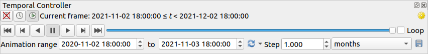
Abb. 7.3 Temporal Controller Panel in navigation mode
 Turn off temporal navigation: all the
temporal settings are disabled and visible layers are rendered as usual
Turn off temporal navigation: all the
temporal settings are disabled and visible layers are rendered as usual Fixed range temporal navigation:
a time range is set and only layers (or features) whose temporal range
overlaps with this range are displayed on the map.
Fixed range temporal navigation:
a time range is set and only layers (or features) whose temporal range
overlaps with this range are displayed on the map. Animated temporal navigation:
a time range is set, split into steps, and only layers (or features)
whose temporal range overlaps with each frame are displayed on the map
Animated temporal navigation:
a time range is set, split into steps, and only layers (or features)
whose temporal range overlaps with each frame are displayed on the map Settings for general control of the animation
Frames rate: number of steps that are shown per second
- Cumulative range: all animation frames will
have the same start date-time but different end dates and times.
This is useful if you wish to accumulate data in your temporal
visualisation instead of showing a ‘moving time window’ across your data.
7.3.3.2. Animating a temporal navigation
An animation is based on a varying set of visible layers at particular times within a time range. To create a temporal animation:
Toggle on the
Animated temporal
navigation, displaying the animation player widgetEnter the Time range to consider. Using the
 button, this can be defined as:
Set to full range of all the time enabled layers
Set to preset project range as defined in the project properties
Set to single layer’s range taken from a time-enabled layer
Fill in the time Step to split the time range. Different units are supported, from
secondstocenturies. Asource timestampsoption is also available as step: when selected, this causes the temporal navigation to step between all available time ranges from layers in the project. It’s useful when a project contains layers with non-contiguous available times, such as a WMS-T service which provides images that are available at irregular dates. This option will allow you to only step between time ranges where the next available image is shown.Click the
 button to preview the animation.
QGIS will generate scenes using the layers rendering at the set times.
Layers display depends on whether they overlap any individual time frame.
button to preview the animation.
QGIS will generate scenes using the layers rendering at the set times.
Layers display depends on whether they overlap any individual time frame.
Abb. 7.4 Temporal navigation through a layer
The animation can also be previewed by moving the time slider. Keeping the
Loop button pressed will repeatedly run the
animation while clicking stops a running animation.
A full set of video player buttons is available.Horizontal scrolling using the mouse wheel (where supported) with the cursor on the map canvas will also allow you to navigate, or “scrub”, the temporal navigation slider backwards and forwards.
Click the
 Export animation button if you want to generate
a series of images representing the scene. They can be later combined in a
video editor software:
Export animation button if you want to generate
a series of images representing the scene. They can be later combined in a
video editor software: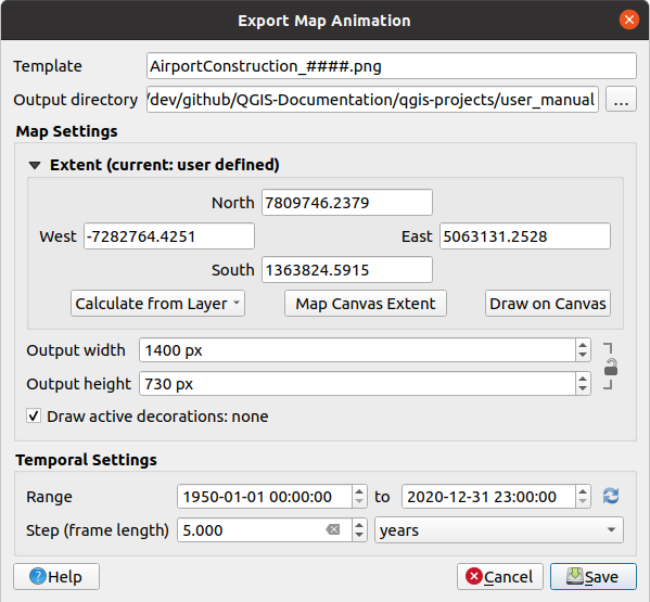
Abb. 7.5 Exporting map canvas animation scenes to images
The filename Template: the
####are replaced with frame sequence numberThe Output directory
Under Map settings, you can:
redefine the spatial extent to use
control the Resolution of the image (Output width and Output height)
Draw active decorations: whether active decorations should be kept in the output
Under Temporal settings, you can redefine:
the time Range for the animation
the Step (frame length) in the unit of your choice
7.3.4. Exporting the map view
Maps you make can be layout and exported to various formats using the advanced capabilities of the print layout or report. It’s also possible to directly export the current rendering, without a layout. This quick „screenshot“ of the map view has some convenient features.
To export the map canvas with the current rendering:
Go to
Depending on your output format, select either
 Export Map to Image…
or
 Export Map to PDF…
The two tools provide you with a common set of options. In the dialog that opens:
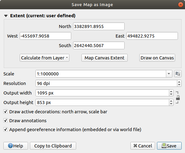
Abb. 7.6 The Save Map as Image dialog
Choose the Extent to export: it can be the current view extent (the default), the extent of a layer or a custom extent drawn over the map canvas. Coordinates of the selected area are displayed and manually editable.
Enter the Scale of the map or select it from the predefined scales: changing the scale will resize the extent to export (from the center).
Set the Resolution of the output
Control the Output width and Output height in pixels of the image: based by default on the current resolution and extent, they can be customized and will resize the map extent (from the center). The size ratio can be locked, which may be particularly convenient when drawing the extent on the canvas.
- Draw active decorations: in use
decorations (scale bar, title, grid, north
arrow…) are exported with the map
- Draw annotations to export any annotation
- Append georeference information (embedded or
via world file): depending on the output format, a world file of
the same name (with extension
PNGWforPNGimages,JPGWforJPG, …) is saved in the same folder as your image. ThePDFformat embeds the information in the PDF file. When exporting to PDF, more options are available in the Save map as PDF… dialog:
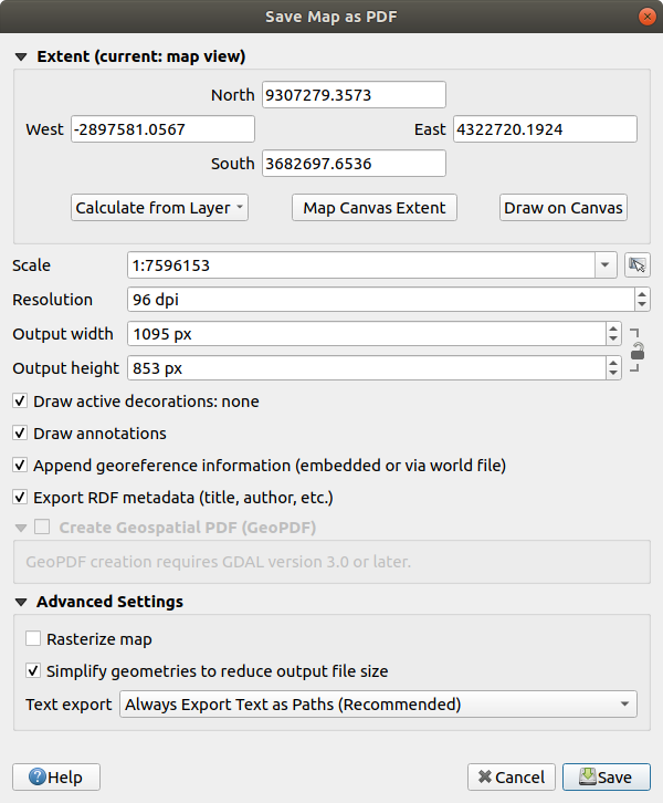
Abb. 7.7 The Save Map as PDF dialog
- Export RDF metadata of the document such
as the title, author, date, description…
- Create Geospatial PDF (GeoPDF):
Generate a
georeferenced PDF file
(requires GDAL version 3 or later).
You can:
Choose the GeoPDF Format
- Include vector feature information in the
GeoPDF file: will include all the geometry and attribute
information from features visible within the map in the output
GeoPDF file.
Bemerkung
Since QGIS 3.10, with GDAL 3 a GeoPDF file can also be used as a data source. For more on GeoPDF support in QGIS, see https://north-road.com/2019/09/03/qgis-3-10-loves-geopdf/.
Rasterize map
- Simplify geometries to reduce output file
size:
Geometries will be simplified while exporting the map by removing
vertices that are not discernably different at the export
resolution (e.g. if the export resolution is
300 dpi, vertices that are less than1/600 inchapart will be removed). This can reduce the size and complexity of the export file (very large files can fail to load in other applications). Set the Text export: controls whether text labels are exported as proper text objects (Always export texts as text objects) or as paths only (Always export texts as paths). If they are exported as text objects then they can be edited in external applications (e.g. Inkscape) as normal text. BUT the side effect is that the rendering quality is decreased, AND there are issues with rendering when certain text settings like buffers are in place. That’s why exporting as paths is recommended.
Click Save to select file location, name and format.
When exporting to image, it’s also possible to Copy to clipboard the expected result of the above settings and paste the map in another application such as LibreOffice, GIMP…
7.4. 3D-Ansicht
3D visualization support is offered through the 3D map view.
You create and open a 3D map view via
 .
A floating QGIS panel will appear. The panel can be docked.
.
A floating QGIS panel will appear. The panel can be docked.
To begin with, the 3D map view has the same extent and view as the 2D main map canvas. A set of navigation tools are available to turn the view into 3D.
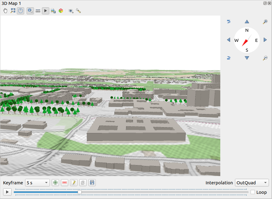
Abb. 7.8 The 3D Map View dialog
The following tools are provided at the top of the 3D map view panel:
- Camera control: moves the view, keeping the same angle
and direction of the camera
- Zoom Full: resizes the view to the whole
layers‘ extent
 Toggle on-screen notification: shows/hides the
navigation widget (that is meant to ease controlling of the map view)
Toggle on-screen notification: shows/hides the
navigation widget (that is meant to ease controlling of the map view) Identify: returns information on the clicked point
of the terrain or the clicked 3D feature(s) – More details at Identifying Features
Identify: returns information on the clicked point
of the terrain or the clicked 3D feature(s) – More details at Identifying Features Measurement line: measures the horizontal distance between points
- Animations: shows/hides the animation player widget
- Save as image…: exports the current view to
an image file format
 Export 3D Scene…: exports the current view as a 3D scene
(
Export 3D Scene…: exports the current view as a 3D scene
(.objfile), allowing post-processing in applications like Blender… The terrain and vector features are exported as 3D objects. The export settings, overriding the layers properties or map view configuration, include:Scene name and destination Folder
Terrain resolution
Terrain texture resolution
Model scale
- Smooth edges
- Export normals
- Export textures
- Set View Theme: Allows you to select the set of layers to
display in the map view from predefined map themes.
- Configure the map view settings
7.4.1. Scene Configuration
The 3D map view opens with some default settings you can customize.
To do so, click the Configure… button at the top of
the 3D canvas panel to open the 3D configuration window.
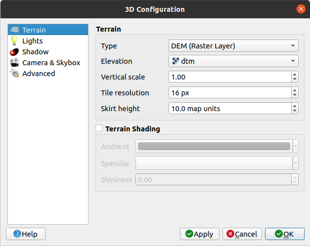
Abb. 7.9 The 3D Map Configuration dialog
In the 3D Configuration window there are various options to fine-tune the 3D scene:
7.4.1.1. Terrain
Terrain: Before diving into the details, it is worth noting that the terrain in a 3D view is represented by a hierarchy of terrain tiles and as the camera moves closer to the terrain, existing tiles that do not have sufficient details are replaced by smaller tiles with more details. Each tile has mesh geometry derived from the elevation raster layer and texture from 2D map layers.
The elevation terrain Type can be:
a Flat terrain
a loaded DEM (Raster Layer)
an Online service, loading elevation tiles produced by Mapzen tools – more details at https://registry.opendata.aws/terrain-tiles/
a loaded Mesh dataset
Elevation: Raster or mesh layer to be used for generation of the terrain. The raster layer must contain a band that represents elevation. For a mesh layer, the Z values of the vertices are used.
Vertical scale: Scale factor for vertical axis. Increasing the scale will exaggerate the height of the landforms.
Tile resolution: How many samples from the terrain raster layer to use for each tile. A value of 16px means that the geometry of each tile will consist of 16x16 elevation samples. Higher numbers create more detailed terrain tiles at the expense of increased rendering complexity.
Skirt height: Sometimes it is possible to see small cracks between tiles of the terrain. Raising this value will add vertical walls („skirts“) around terrain tiles to hide the cracks.
Terrain elevation offset: moves the terrain up or down, e.g. to adjust its elevation with respect to the ground level of other objects in the scene.
This can be useful when there is a discrepancy between the height of the terrain and the height of layers in your scene (e.g. point clouds which use a relative vertical height only). In this case adjusting the terrain elevation manually to coincide with the elevation of objects in your scene can improve the navigation experience.
When a mesh layer is used as terrain, you can configure the Triangles settings (wireframe display, smooth triangles, level of detail) and the Rendering colors settings (as a uniform color or color ramp based). More details in the Mesh layer 3D properties section.
- Terrain shading: Allows you to choose how the
terrain should be rendered:
Shading disabled - terrain color is determined only from map texture
Shading enabled - terrain color is determined using Phong’s shading model, taking into account map texture, the terrain normal vector, scene light(s) and the terrain material’s Ambient and Specular colors and Shininess
7.4.1.2. Lights
From the Lights tab, press the  menu to add
up to eight Point lights: emits light in all directions, like a sphere of light filling an area. Objects closer to the light will be brighter, and objects further away will be darker. A point light has a set position (X, Y and Z), a Color, an Intensity and an Attenuation
up to four Directional lights: mimics the lighting that you would get from a giant flash light very far away from your objects, always centered and that never dies off (e.g. the sun). It emits parallel light rays in a single direction but the light reaches out into infinity. A directional light can be rotated given an Azimuth, have an Altitude, a Color and an Intensity.
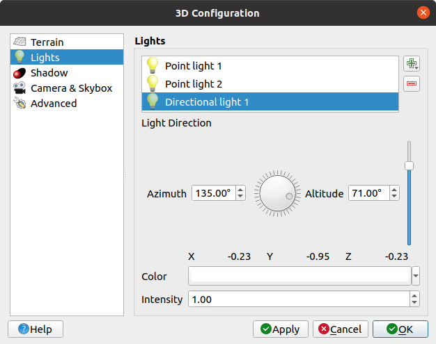
Abb. 7.10 The 3D Map Lights Configuration dialog
7.4.1.3. Shadow
Check Show shadow to display shadow within your scene,
given:
a Directional light
a Shadow rendering maximum distance: to avoid rendering shadow of too distant objects, particularly when the camera looks up along the horizon
a Shadow bias: to avoid self-shadowing effects that could make some areas darker than others, due to differences between map sizes. The lower the better
a Shadow map resolution: to make shadows look sharper. It may result in less performance if the resolution parameter is too high.
7.4.1.4. Camera & Skybox
In this tab, you can override some default camera settings made in the dialog.
Furthermore, check Show skybox to enable skybox rendering
in the scene. The skybox type can be:
Panoramic texture, with a single file providing sight on 360°
Distinct faces, with a texture file for each of the six sides of a box containing the scene
Texture image files of the skybox can be files on the disk, remote URLs or embedded in the project (more details).
7.4.1.5. Advanced
Map tile resolution: Width and height of the 2D map images used as textures for the terrain tiles. 256px means that each tile will be rendered into an image of 256x256 pixels. Higher numbers create more detailed terrain tiles at the expense of increased rendering complexity.
Max. screen error: Determines the threshold for swapping terrain tiles with more detailed ones (and vice versa) - i.e. how soon the 3D view will use higher quality tiles. Lower numbers mean more details in the scene at the expense of increased rendering complexity.
Max. ground error: The resolution of the terrain tiles at which dividing tiles into more detailed ones will stop (splitting them would not introduce any extra detail anyway). This value limits the depth of the hierarchy of tiles: lower values make the hierarchy deep, increasing rendering complexity.
Zoom levels: Shows the number of zoom levels (depends on the map tile resolution and max. ground error).
- Show labels: Toggles map labels on/off
- Show map tile info: Include border and tile
numbers for the terrain tiles (useful for troubleshooting terrain
issues)
- Show bounding boxes: Show 3D bounding boxes
of the terrain tiles (useful for troubleshooting terrain issues)
- Show camera’s view center
- Show light sources: shows a sphere at light source
origins, allowing easier repositioning and placement of light sources relative
to the scene contents
7.4.2. Navigation options
To explore the map view in 3D:
Tilt the terrain (rotating it around a horizontal axis that goes through the center of the window)
Press the
 Tilt up and
  Tilt down tools
Press Shift and use the up/down keys
Ziehen Sie die Maus bei gedrückter mittlerer Maustaste vorwärts/rückwärts.
Drücken Sie Shift und ziehen Sie die Maus mit gedrückter linker Maustaste vorwärts/rückwärts.
Rotate the terrain (around a vertical axis that goes through the center of the window)
Turn the compass of the navigation widget to the watching direction
Press Shift and use the left/right keys
Drag the mouse right/left with the middle mouse button pressed
Press Shift and drag the mouse right/left with the left mouse button pressed
Change the camera position (and the view center), moving it around in a horizontal plan
Drag the mouse with the left mouse button pressed, and the
Camera control button enabledPress the directional arrows of the navigation widget
Use the up/down/left/right keys to move the camera forward, backward, right and left, respectively
Change the camera altitude: press the Page Up/Page Down keys
Change the camera orientation (the camera is kept at its position but the view center point moves)
Press Ctrl and use the arrow keys to turn the camera up, down, left and right
Press Ctrl and drag the mouse with the left mouse button pressed
Zoom in and out
Press the corresponding
Zoom In and
Zoom Out tools of the navigation widgetScroll the mouse wheel (keep Ctrl pressed results in finer zooms)
Drag the mouse with the right mouse button pressed to zoom in (drag down) and out (drag up)
To reset the camera view, click the Zoom Full
button on the top of the 3D canvas panel.
7.4.3. Creating an animation
An animation is based on a set of keyframes - camera positions at particular times. To create an animation:
Toggle on the
Animations tool, displaying the animation player
widgetClick the
Add keyframe button and enter a Keyframe
time in seconds. The Keyframe combo box now displays the time set.Using the navigation tools, move the camera to the position to associate with the current keyframe time.
Repeat the previous steps to add as many keyframes (with time and position) as necessary.
Click the
button to preview the animation. QGIS will generate scenes using
the camera positions/rotations at set times, and interpolating them in between
these keyframes. Various Interpolation modes for animations are
available (eg, linear, inQuad, outQuad, inCirc… – more details at
https://doc.qt.io/qt-5/qeasingcurve.html#EasingFunction-typedef).The animation can also be previewed by moving the time slider. Keeping the Loop box checked will repeatedly run the animation while clicking
stops a running animation.
Click Export animation frames to generate a series of images
representing the scene. Other than the filename Template and the
Output directory, you can set the number of Frames per
second, the Output width and Output height.
7.4.4. 3D vector layers
A vector layer with elevation values can be shown in the 3D map view by checking Enable 3D Renderer in the 3D View section of the vector layer properties. A number of options are available for controlling the rendering of the 3D vector layer.
7.5. Statusleiste
The status bar provides you with general information about the map view and processed or available actions, and offers you tools to manage the map view.
7.5.1. Locator bar
On the left side of the status bar, the locator bar, a quick search widget, helps you find and run any feature or options in QGIS:
Click in the text widget to activate the locator search bar or press Ctrl+K.
Type a text associated with the item you are looking for (name, tag, keyword, …). By default, results are returned for the enabled locator filters, but you can limit the search to a certain scope by prefixing your text with the locator filters prefix, ie. typing
l cadwill return only the layers whose name containscad.The filter can also be selected with a double-click in the menu that shows when accessing the locator widget.
Click on a result to execute the corresponding action, depending on the type of item.
Tipp
Limit the lookup to particular field(s) of the active layer
By default, a search with the „active layer features“ filter (f) runs
through the whole attribute table of the layer. You can limit the search to
a particular field using the @ prefix. E.g., f @name sal or
@name sal returns only the features whose „name“ attribute contains ‚sal‘.
Text autocompletion is active when writing and the suggestion can be applied
using Tab key.
A more advanced control on the queried fields is possible from the layer Fields tab. Read Fields Properties for details.
Searching is handled using threads, so that results always become available as quickly as possible, even if slow search filters are installed. They also appear as soon as they are encountered by a filter, which means that e.g. a file search filter will show results one by one as the file tree is scanned. This ensures that the UI is always responsive, even if a very slow search filter is present (e.g. one which uses an online service).
Bemerkung
The Nominatim locator tool may behave differently (no autocompletion search, delay of fetching results, …) with respect to the OpenStreetMap Nominatim usage policy.
Tipp
Quick access to the locator’s configurations
Click on the  icon inside the locator widget on the status bar to
display the list of filters you can use and a Configure entry that
opens the Locator tab of the menu.
icon inside the locator widget on the status bar to
display the list of filters you can use and a Configure entry that
opens the Locator tab of the menu.
7.5.2. Reporting actions
In the area next to the locator bar, a summary of actions you’ve carried out will be shown when needed (such as selecting features in a layer, removing layer, pan distance and direction) or a long description of the tool you are hovering over (not available for all tools).
In case of lengthy operations, such as gathering of statistics in raster layers, executing Processing algorithms or rendering several layers in the map view, a progress bar is displayed in the status bar.
7.5.3. Control the map canvas
The ![]() Coordinate option shows the current
position of the mouse, following it while moving across the map view.
You can set the units (and precision) in the
tab.
Click on the small button at the left of the textbox to toggle between
the Coordinate option and the
Coordinate option shows the current
position of the mouse, following it while moving across the map view.
You can set the units (and precision) in the
tab.
Click on the small button at the left of the textbox to toggle between
the Coordinate option and the  Extents option
that displays the coordinates of the current bottom-left and top-right
corners of the map view in map units.
Extents option
that displays the coordinates of the current bottom-left and top-right
corners of the map view in map units.
Next to the coordinate display you will find the Scale display. It shows the scale of the map view. There is a scale selector, which allows you to choose between predefined and custom scales.
On the right side of the scale display, press the  button
to lock the scale to use the magnifier to zoom in or out.
The magnifier allows you to zoom in to a map without altering the map
scale, making it easier to tweak the positions of labels and symbols
accurately.
The magnification level is expressed as a percentage.
If the Magnifier has a level of 100%, then the current map
is not magnified, i.e. is rendered at accurate scale relative to the monitor’s resolution (DPI).
A default magnification value can be defined within
,
which is very useful for high-resolution screens to enlarge small
symbols. In addition, a setting in
controls whether QGIS respects each monitor’s physical DPI or uses the overall system logical DPI.
button
to lock the scale to use the magnifier to zoom in or out.
The magnifier allows you to zoom in to a map without altering the map
scale, making it easier to tweak the positions of labels and symbols
accurately.
The magnification level is expressed as a percentage.
If the Magnifier has a level of 100%, then the current map
is not magnified, i.e. is rendered at accurate scale relative to the monitor’s resolution (DPI).
A default magnification value can be defined within
,
which is very useful for high-resolution screens to enlarge small
symbols. In addition, a setting in
controls whether QGIS respects each monitor’s physical DPI or uses the overall system logical DPI.
To the right of the magnifier tool you can define a current clockwise rotation for your map view in degrees.
On the right side of the status bar, there is a small checkbox which can be used temporarily to prevent layers being rendered to the map view (see section Layeranzeige kontrollieren).
To the right of the render functions, you find the  EPSG:code button showing the current project CRS. Clicking
on this opens the Project Properties dialog and lets you
apply another CRS to the map view.
EPSG:code button showing the current project CRS. Clicking
on this opens the Project Properties dialog and lets you
apply another CRS to the map view.
Tipp
Die richtige Maßstabseinheit im Kartenfenster einstellen
When you start QGIS, the default CRS is WGS 84 (EPSG 4326) and
units are degrees. This means that QGIS will interpret any
coordinate in your layer as specified in degrees.
To get correct scale values, you can either manually change this
setting in the General tab under
(e.g. to meters), or you
can use the EPSG:code icon seen above.
In the latter case, the units are set to what the project projection
specifies (e.g., +units=us-ft).
Beachten Sie, dass die KBS Wahl beim Start unter eingestellt werden kann.
7.5.4. Messaging
The  Messages button next to it opens the
Log Messages Panel which has information on underlying
processes (QGIS startup, plugins loading, processing tools…)
Messages button next to it opens the
Log Messages Panel which has information on underlying
processes (QGIS startup, plugins loading, processing tools…)
Depending on the Plugin Manager settings,
the status bar can sometimes show icons to the right to inform you
about the availability of new ( ) or upgradeable (
 )
plugins.
Click the icon to open the Plugin Manager dialog.
)
plugins.
Click the icon to open the Plugin Manager dialog.