20. Werken met puntenwolken

20.1. Introductie voor puntenwolken

Wat is een puntenwolk?

Een puntenwolk is een drie-dimensionale afbeelding van een ruimte die is opgemaakt door heel veel individuele gegevenspunten (meer dan biljoenen, zelfs triljoenen). Elk van de punten heeft een X, Y en Z-coördinaat. Afhankelijk van de methode van vastleggen hebben puntenwolken gewoonlijk ook aanvullende attributen die komen uit het vastleggen, zoals kleurwaarden of intensiteit. Deze attributen kunnen worden gebruikt, bijvoorbeeld, om puntenwolken in verschillende kleuren weer te geven. In QGIS kan een puntenwolk worden gebruikt om een drie-dimensionale afbeelding van het landschap (of een andere ruimte) te maken.

Ondersteunde indelingen

QGIS ondersteunt de indelingen voor gegevens Entwine Point Tile (EPT) en LAS/LAZ. QGIS slaat, bij het werken met puntenwolken, de gegevens altijd op in EPT. EPT is een indeling voor opslag die bestaat uit verschillende bestanden, opgeslagen in een gedeelde map. EPT gebruikt indexeren om snelle toegang tot de gegevens mogelijk te maken. Voor meer informatie over de indeling EPT, bekijk Entwine homepage

Als de gegevens in de indelingen LAS of LAZ staan, zal QGIS ze converteren naar EPT wanneer ze voor de eerste keer worden geladen. Afhankelijk van de grootte van het bestand zou dit enige tijd kunnen vergen. In dit proces wordt een submap gemaakt in de map waar het bestand LAS/LAZ is geplaatst, overeenkomstig het schema ept_ + name_LAS/LAZ_file. Als een dergelijke map al bestaat, laadt QGIS het EPT onmiddellijk (wat leidt tot een verkorte tijd voor het laden).

Goed om te weten

In QGIS is het (nog) niet mogelijk om puntenwolken te bewerken. Als u uw puntenwolk wilt bewerken kunt u CloudCompare gebruiken, een open bron programma voor het bewerken van puntenwolken. Ook de Point Data Abstraction Library (PDAL - soortgelijk aan GDAL) biedt u opties om puntenwolken te bewerken (PDAL is alleen voor de opdrachtregel).

Vanwege het grote aantal gegevenspunten is het niet mogelijk om een attributentabel van puntenwolken weer te geven in QGIS. Echter, het gereedschap Objecten identificeren ondersteunt puntenwolken, dus kunt u alle attributen weergeven, zelfs van één enkel gegevenspunt.

20.2. Eigenschappen Puntenwolken

Het dialoogvenster Laageigenschappen voor een laag met een puntenwolk biedt algemene instellingen voor de laag en het renderen ervan. Het verschaft ook informatie over de laag.

Toegang tot het dialoogvenster Laag-eigenschappen:

• In het paneel Lagen, dubbelklik op de laag of klik met rechts en selecteer Eigenschappen… uit het contextmenu;

• Ga naar menu Kaartlagen ► Laageigenschappen… als de laag is geselecteerd.

Het puntenwolk dialoogvenster Laageigenschappen verschaft de volgende gedeelten:

Informatie	Bron	Symbologie[1]
3D-weergave[1]	Renderen	Hoogte[1]
Metadata	Statistieken

^[1] Ook beschikbaar in het paneel Laag opmaken

Notitie

De meeste eigenschappen van een puntenwolk laag kan worden opgeslagen naar of geladen uit een bestand .qml met het menu Stijl aan de onderzijde van het dialoogvenster voor de eigenschappen. Meer details in Laageigenschappen opslaan en delen

20.2.1. Eigenschappen Informatie

De tab Informatie is alleen-lezen en is een interessante plek om snel wat overzichtsinformatie en metadata over de huidige laag op te pakken. Verschafte informatie is:

• Algemeen, zoals naam in het project, pad van de bron, laatste tijd en grootte van opslaan, de gebruikte provider

• Gebaseerd op de provider van de laag: bereik en aantal punten

• Het Coördinaten ReferentieSysteem: naam, eenheden, methode, nauwkeurigheid, verwijzing (d.i. of het statisch of dynamisch is)

• Metadata geleverd door de provider: datum van maken, versie, indeling gegevens, schaal X/Y/Z, …

• Gekozen vanaf de tab Metadata (waar zij kunnen worden bewerkt): toegang, bereiken, links, contacten, geschiedenis…

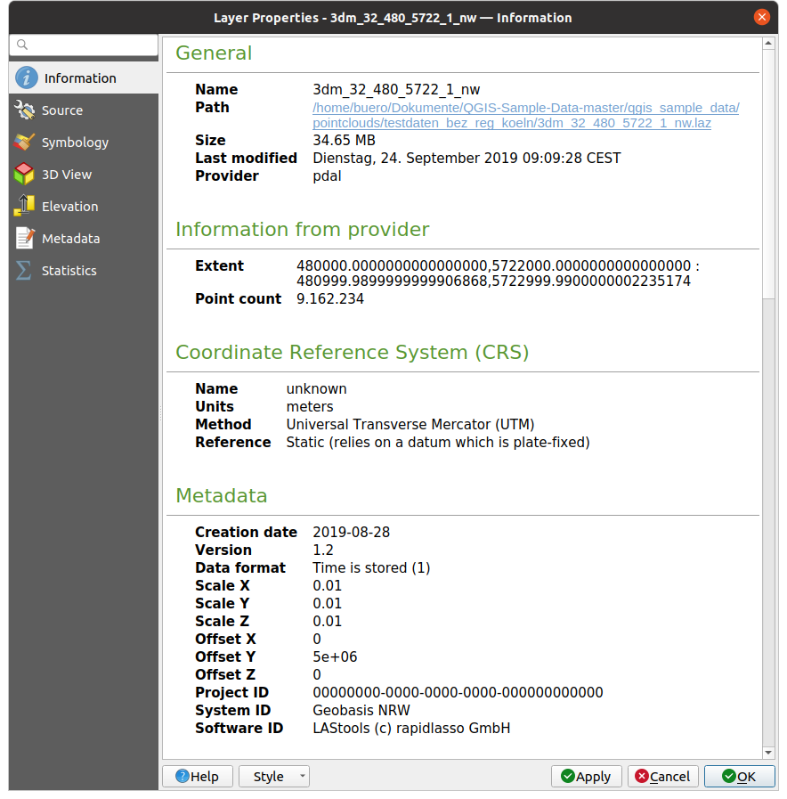
Fig. 20.1 Puntenwolk tab Informatie

20.2.2. Eigenschappen Bron

Op de tab Bron kunt u basisinformatie over de puntenwolk laag bekijken en bewerken:

• Instellingen: Stel een Laagnaam in die anders is dan de bestandsnaam van de laag die zal worden gebruikt om de laag in het project te identificeren (in het Paneel Lagen, met expressies, in de legenda van de afdruklay-out, …)

• Toegewezen Coördinaten ReferentieSysteem (CRS): Hier kunt u het aan de laag toegewezen Coördinaten ReferentieSysteem wijzigen. door een recent gebruikte te selecteren uit de keuzelijst of te klikken op de knop CRS selecteren (bekijk Keuze Coördinaten ReferentieSysteem). Gebruik dit proces alleen als het op de laag toegepaste CRS verkeerd is of als er geen werd gespecificeerd.

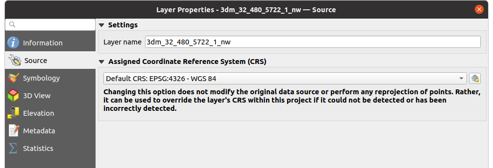
Fig. 20.2 Puntenwolk tab Bron

20.2.3. Eigenschappen Symbologie

Op de tab Symbologie worden de instellingen voor het renderen van de puntenwolk. In het bovenste gedeelte zijn de instellingen voor de verschillende renderers voor de objecten te vinden. In het onderste gedeelte zijn er delen waarmee algemene instellingen voor de gehele laag kunnen worden gemaakt en die voorrang hebben boven renderers voor objecten.

20.2.3.1. Typen renderer voor objecten

Er zijn verschillende opties voor het renderen van puntenwolken die kunnen worden geselecteerd met het keuzemenu aan de bovenzijde van de tab Symbologie (zie Fig. 20.3):

• Alleen bereik: Alleen een begrenzingsvak van het bereik van de gegevens wordt weergegeven; handig voor een overzicht van het bereik van de gegevens. Zoals gewoonlijk helpt de widget Symbool u de eigenschappen te configureren (kleur, dikte, opaciteit, sub-lagen, …) die u wilt voor het vak.

• Attributen per kleurverloop: De gegevens worden getekend met een kleurverloop. Bekijk Renderer Attributen per kleurverloop

• RGB: Teken de gegevens met waarden voor de kleuren rood, groen en blauw. Bekijk Renderer RGB

• Classificatie: De gegevens worden getekend met verschillende kleuren voor verschillende klassen. Bekijk Renderer Classificatie

Wanneer een puntenwolk wordt geladen volgt QGIS logica om de beste renderer te selecteren:

• als de gegevensset informatie over kleuren bevat (attributen rood, groen, blauw), zal de renderer RGB worden gebruikt

• anders als de gegevensset een attribuut Classificatie bevat, zal de renderer Classificatie worden gebruikt

• anders valt het terug op renderen dat is gebaseerd op het attribuut Z

Als u de attributen van de puntenwolk niet weet verschaft de tab Statistieken een goed overzicht van welke attributen zijn opgenomen in de puntenwolk en in welke bereiken de waarden zijn geplaatst.

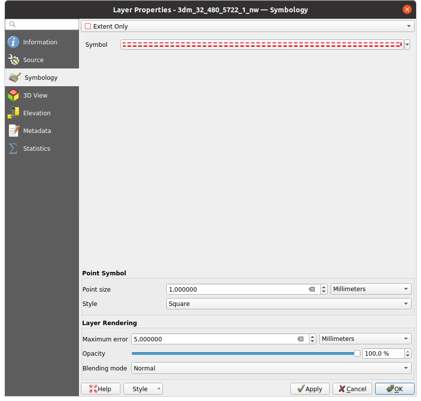
Fig. 20.3 Puntenwolk tab Symbologie

Renderer Attributen per kleurverloop

Met Attributen per kleurverloop, kunnen de gegevens worden weergegeven op numerieke waarden met behulp van een kleurverloop. Zulke numerieke waarden kunnen, bijvoorbeeld, een bestaand attribuut Intensity of de waarde Z zijn. Afhankelijk van een minimum en een maximum waarde, worden de andere waarden over het kleurverloop verspreid via interpolatie. De afzonderlijke waarden en hun toewijzing aan een bepaalde kleur worden “kleurenkaart” genoemd en worden in de tabel weergegeven. Er zijn verschillende opties voor instellingen, die onder de afbeelding beschreven worden.

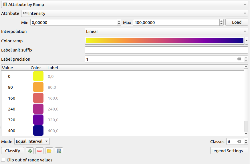
Fig. 20.4 Puntenwolk tab Symbologie: Attributen per kleurverloop

• Min en Max definiëren het bereik dat wordt toegepast op het kleurverloop: de waarde Min geeft het linker einde, de waarde Max het rechter einde van het kleurverloop weer, de waarden daartussen worden geïnterpoleerd. Standaard detecteert QGIS minimum en maximum uit het geselecteerde attribuut, maar zij kunnen worden aangepast. Als u de waarden eenmaal hebt gewijzigd, kunt u de standaard herstellen door te klikken op de knop Laden.

• Het item Interpolatie definieert hoe waarden hun kleur krijgen toegewezen:

  • Afzonderlijk (een symbool <= verschijnt in de kop van de kolom Waarde): De kleur wordt genomen uit het dichtstbijzijnde item van de kleurenkaart met een gelijke of hogere waarde

  • Lineair: De kleur wordt lineair geïnterpoleerd uit de items van de kleurenkaart boven en onder de pixelwaarde, wat betekent dat elke waarde van de gegevensset correspondeert met een unieke kleur

  • Exact (een symbool = verschijnt in de kop van de kolom Waarde): Alleen op pixels met een waarde die gelijk is aan een item van de kleurenkaart wordt een kleur toegepast; andere worden niet gerenderd.

• De widget Kleurverloop helpt u het aan de gegevensset toe te wijzen kleurverloop te selecteren. Zoals gewoonlijk met dit widget, kunt u een nieuwe maken en bewerken of het huidige geselecteerde opslaan.

• Het Label voor achtervoegsel eenheid voegt een label toe na de waarde in de legenda, en de Precisie label beheert het aantal decimalen dat moet worden weergegeven.

De classificatie Modus helpt u te definiëren hoe waarden over de klassen worden verdeeld:

• Doorgaand: Aantal en kleur van de klassen worden opgehaald uit de stappen van het kleurverloop; grenswaarden worden ingesteld naar aanleiding van de verdeling van de stops in het kleurverloop (u kunt meer informatie over stops vinden in Een kleurverloop instellen)..

• Gelijke interval: het aantal klassen wordt ingesteld door het veld Klassen; grenzen van waarden worden gedefinieerd, zodat de klassen allemaal dezelfde grootte hebben.

De klassen worden automatisch bepaald en weergegeven in de tabel met kleuren. Maar u kunt deze klassen ook handmatig bewerken:

• Dubbelklikken op een Waarde in de tabel: laat u de waarde van de klasse aanpassen.

• Dubbelklikken in de kolom Kleur opent de widget Kleur selecteren, waar u een kleur kunt selecteren om toe te passen op die waarde

• Dubbelklikken in de kolom Label laat u het label van de klasse aanpassen

• Met rechts klikken op geselecteerde rijen in de kleurentabel geeft een contextmenu weer om Kleur wijzigen… en Opaciteit wijzigen… voor de selectie.

Onder de tabel staan de opties om de standaard klassen te herstellen met Classificeren of om handmatig waarden ^{Toe te voegen} of geselecteerde waarden te ^Verwijderen uit de tabel.

Omdat een aangepaste kleurenkaart zeer complex kan zijn is er ook de optie om een bestaande kleurenkaart te ^Laden of voor het ^Opslaan om in andere lagen te gebruiken (als een bestand txt).

Als u Lineair hebt geselecteerd voor Interpolatie kunt u ook configureren:

• Clip buiten bereik van waarden Standaard wijst de methode Lineair de kleur van de eerste klasse (respectievelijk de laatste klasse) toe aan waarden in de gegevensset die kleiner zijn dan de ingestelde waarde Min (respectievelijk groter dan het ingestelde Max). Selecteer deze instelling als u deze waarden niet wilt renderen.

• Instellingen Legenda voor het weergeven in het paneel Lagen en in het lay-out item Legenda. Aanpassen werkt hetzelfde als voor een rasterlaag (Vind meer details op Legenda van raster aanpassen).

Renderer RGB

Met de renderer RGB zullen drie geselecteerde attributen uit de puntenwolk worden gebruikt als de rode, groene en blauwe component. Als de attributen overeenkomstig worden benoemd, selecteert QGIS ze automatisch en haalt de waarden Min en Max voor elke band op en brengt de kleur overeenkomstig op schaal. Het is echter ook mogelijk de waarden handmatig aan te passen.

Een methode voor Contrastverbetering kan worden toegepast voor de waarden: Geen verbetering, Stretch tot MinMax, Stretch e clip tot MinMax en Clip naar MinMax

Notitie

Het gereedschap Contrastverbetering is nog steeds in ontwikkeling. Als u er problemen mee hebt, zou u de standaard instelling Stretch tot MinMax moeten gebruiken.

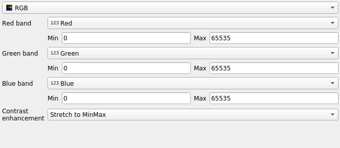
Fig. 20.5 De puntenwolk renderer RGB

Renderer Classificatie

Met de renderer Classificatie wordt de puntenwolk weergegeven met een verschil in kleur op basis van een attribuut. Elk type attribuut mag worden gebruikt (numeriek, tekenreeks, …). Gegevens van puntenwolken bevatten vaak een veld genaamd Classificatie. Dat bevat doorgaans gegevens die automatisch kunnen worden bepaald door nabewerken, bijv. over vegetatie. Met Attribuut kunt u het veld selecteren uit de attributentabel dat zal worden gebruikt voor de classificatie. Standaard gebruikt QGIS de definities van de specificatie van LAS (bekijk de tabel ‘ASPRS Standard Point Classes’ in de PDF op ASPRS homepage). De gegevens kunnen echter afwijken van dit schema; in geval van twijfel, zult u naar de definities moeten vragen aan degene of het instituut waar u de gegevens van hebt ontvangen.

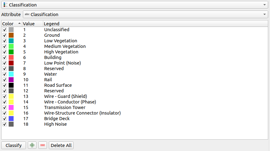
Fig. 20.6 De puntenwolk renderer Classificatie

In de tabel worden alle gebruikte waarden weergegeven met de corresponderende kleur en legenda. Aan het begin van elke rij staat een keuzevak ; als dat niet is geselecteerd wordt deze waarde niet langer weergegeven op de kaart. Met een dubbelklik in de tabel kunnen de Kleur, de Waarde en de Legenda worden aangepast (voor de kleur opent de widget Kleur selecteren).

Onder de tabel staan knoppen waarmee u de standaard klassen, gemaakt door QGIS, kunt wijzigen:

• Met de knop Classificeren kunnen de gegevens automatisch worden geclassificeerd: alle waarden die voorkomen in de attributen en nog niet in de tabel staan worden toegevoegd

• Met ^Toevoegen en ^Verwijderen kunnen waarden handmatig worden toegevoegd of verwijderd

• Alles verwijderen verwijdert alle waarden uit de tabel

Hint

In het paneel Lagen kunt u met rechts klikken op een item van een klasse van een laag om snel de zichtbaarheid van de overeenkomende objecten te configureren.

20.2.3.2. Puntsymbool

Onder Puntsymbool, kunnen de grootte en eenheid (bijv. millimeters, pixels, inches) waarmee elk gegevenspunt wordt weergegeven worden ingesteld. Ofwel Cirkel of Vierkant kan worden geselecteerd als de stijl voor de punten.

20.2.3.3. Renderen van lagen

In het gedeelte Renderen van lagen heeft u de volgende opties om het renderen van de laag aan te passen:

• Tekenvolgorde: maakt het mogelijk te beheren of de volgorde van renderen voor puntenwolken op 2D-kaartvenster zou moeten bepaald op het waarde Z. Het is mogelijk te renderen :

  • in de volgorde Standaard waar de punten mee zijn opgeslagen in de laag,

  • met Van beneden naar boven (punten met een grotere waarde Z bedekken lagere punten, wat het uiterlijk van een echte ortho-foto geeft),

  • of met Van boven naar beneden waarmee de scene verschijnt als wordt hij van onder bekeken.

• Maximum fout: Puntenwolken bevatten gewoonlijk meer punten dan nodig zijn voor het weergeven. Met deze optie stelt u in hoe dicht of schraal de weergave van de puntenwolk zal zijn (dit kan ook worden begrepen als ‘maximale toegestane gat tussen punten’). Als u een hoog getal invoert (bijv. 5 mm), zullen er zichtbare gaten tussen de punten zijn. Lage waarde (bijv. 0.1 mm) zou het renderen van een onnodig aantal punten kunnen forceren, wat het renderen trager maakt (verschillende eenheden kunnen worden geselecteerd).

• Opaciteit: U kunt hiermee onderliggende lagen zichtbaar maken in het kaartvenster. Gebruik de schuifbalk om de transparantie van de geselecteerde vectorlaag aan te passen naar uw behoeften. U kunt ook een precieze definitie voor het percentage voor de transparantie invullen in het menu naast de schuifbalk.

• Meng-modus: Met dit gereedschap kunt u speciale effecten op de kaart toepassen. De pixels van de overliggende en onderliggende lagen worden vermengd volgens de instellingen zoals beschreven in Meng-modi.

• Eye dome lighting: dit past effecten voor schaduw toe op het kaartvenster voor het beter renderen van de diepte. Kwaliteit van het renderen is afhankelijk van de eigenschap tekenvolgorde; de tekenvolgorde Standaard zou sub-optimale resultaten kunnen geven. De volgende parameters kunnen worden beheerd:

  • Sterkte: vergroot het contrast, maakt een betere perceptie voor diepte mogelijk

  • Afstand: geeft de afstand weer tussen de gebruikte pixels vanaf de pixel van het middelpunt en heeft het effect van het dikker maken van de randen.

20.2.4. Eigenschappen 3D-weergave

Op de tab 3D-weergave kunt u de instellingen maken voor het renderen van de puntenwolk in 3D-kaarten.

20.2.4.1. Modi 3D renderen

De volgende opties kunnen worden geselecteerd uit het keuzemenu aan de bovenzijde van de tab:

• Niet renderen: Gegevens worden niet weergegeven

• 2D-symbologie volgen: Synchroniseert objecten bij het renderen in 3D met symbologie die is toegewezen voor 2D

• Enkele kleur: Alle punten worden weergegeven in dezelfde kleur ongeacht hun attributen

• Attributen per kleurverloop: Interpoleert een opgegeven attribuut over een kleurverloop en wijst de objecten hun overeenkomende kleur toe. Bekijk Renderer Attributen per kleurverloop

• RGB: Gebruik verschillende attributen van de objecten om de kleurcomponenten Rood, Groen en Blauw in te stellen om ze toe te kunnen wijzen. Bekijk Renderer RGB.

• Classificatie: Differentieert punten op hun kleur op basis van een attribuut Bekijk Renderer Classificatie.

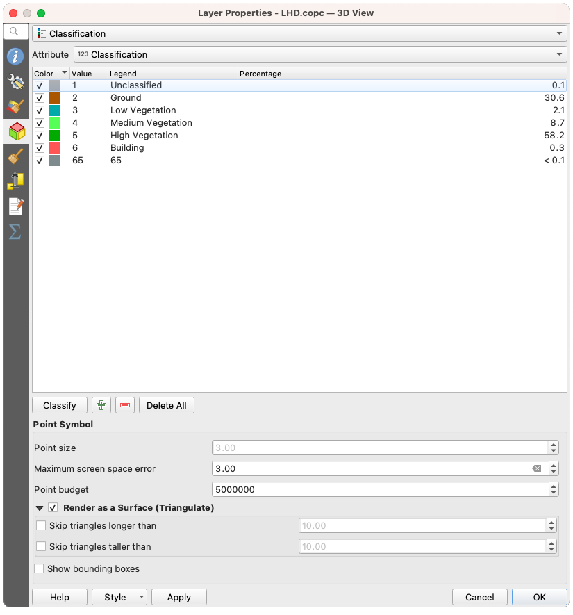
Fig. 20.7 De puntenwolk tab 3D-weergave met de renderer Classificatie

20.2.4.2. 3D-puntsymbool

In het onderste gedeelte van de tab 3D-weergave vindt u het gedeelte Puntsymbool. Hier kunt u voor de gehele laag algemene instellingen maken die hetzelfde zijn voor alle renderers. Er zijn de volgende opties:

• Grootte punt: De grootte (in pixels) waarmee elk gegevenspunt wordt weergegeven kan worden ingesteld

• Max. schermruimte fout: Met deze optie stelt u in hoe dicht of schraal de weergave van de puntenwolk zal zijn (in pixels). Als u een groot getal instelt (bijv. 10), zullen er zichtbare gaten tussen de punten zijn; lage waarde (bijv. 0) zou renderen van een onnodig aantal punten kunnen forceren, wat het renderen trager maakt (u kunt meer details vinden in Symbologie Maximum fout).

• Budget punt: U kunt het maximale aantal te renderen punten instellen om lang renderen te vermijden

• Selecteer Renderen als oppervlakte (Trianguleren) om de laag van de puntenwolk in de 3D-weergave te renderen met een gevuld oppervlak, verkregen uit triangulatie. U kunt de dimensies van de berekende driehoeken beheren:

  • Driehoeken overslaan die langer zijn dan een drempelwaarde: stelt het horizontale vlak in, de maximale lengte van een zijde van de driehoeken om rekening mee te houden

  • Driehoeken overslaan die groter zijn dan een drempelwaarde: stelt het verticale vlak in, de maximale hoogte van een zijde van de driehoeken om rekening mee te houden

• Begrenzingsvakken tonen: Speciaal nuttig bij debuggen, geeft de begrenzingsvakken van knopen weer in hiërarchie

20.2.5. Rendering

Onder het groepsvak Schaalafhankelijke zichtbaarheid, kunt u de schaal Maximum (inclusief) en Minimum (exclusief) instellen, wat een bereik van schalen definieert waarin objecten zichtbaar zullen zijn. Buiten dit bereik is hij verborgen. De knop ^{Op huidige schaal kaartvenster instellen} helpt u de schaal van het huidige kaartvenster te gebruiken als grens voor de zichtbaarheid van het bereik. Bekijk Schaal zichtbaarheid selecteren voor meer informatie.

Notitie

U kunt het schaalafhankelijk renderen ook activeren op een laag vanuit het paneel Lagen. Klik met rechts op de laag en selecteer in het contextmenu, Zichtbaarheidsschaal laag instellen.

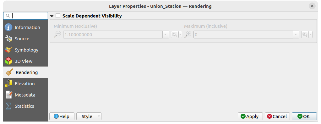
Fig. 20.8 De puntenwolk tab Renderen

20.2.6. Eigenschappen hoogte

Op de tab Hoogte kunt u correcties instellen voor de waarden Z van de gegevens. Dit zou nodig kunnen zijn om de hoogte van de gegeven in 3D-kaarten aan te passen en het uiterlijk in de diagrammen van het profiel. Er zijn twee opties voor de instelling:

• Onder de groep Hoogte:

  • U kunt een Schaal instellen: Als 10 hier wordt ingevoerd zal een punt, dat een waarde Z = 5 heeft, worden weergegeven op een hoogte van 50.

  • Een Verschuiving naar het niveau Z kan worden ingevoerd. Dit is nuttig om verschillende databronnen, ten opzichte van elkaar, in hoogte overeen te laten komen. Standaard wordt de laagste waarde Z die is opgenomen in de gegevens als deze waarde gebruikt. Deze waarde kan ook worden hersteld met de knop ^Vernieuwen aan het einde van de regel.

• Under Nauwkeurigheid diagram profiel, de Maximum fout helpt u beheren hoe dicht of schaarser bij elkaar de punten zullen worden gerenderd in het hoogteprofiel. Grotere waarden resulteren in een sneller maken met minder opgenomen punten.

• Onder Uiterlijk diagram profiel kunt u de weergave van de punten beheren:

  • Grootte punt: de grootte waarmee de punten gerenderd moeten worden, in ondersteunde eenheden (millimeters, kaarteenheden, pixels, …)

  • Stijl: of de punten als Cirkel of Vierkant moeten worden gerenderd

  • Pas één enkele Kleur toe op alle zichtbare punten in de weergave van het profiel

  • Selecteer Kleur laag respecteren om in plaats daarvan de punten weer te geven met de in hun 2D symbology toegewezen kleur

  • Opaciteit bij afstand effect van boog toepassen verklein de opaciteit van punten die verder weg liggen van boog van het profiel

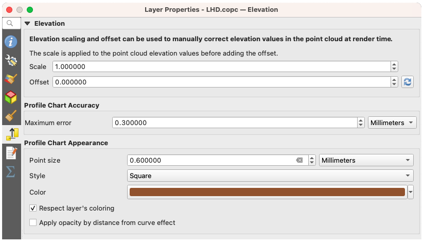
Fig. 20.9 De puntenwolk tab Hoogte

20.2.7. Metadata

De tab Metadata verschaft u opties om een rapport met metadata voor uw laag te maken en te bewerken. Bekijk Metadata voor meer informatie.

20.2.8. Eigenschappen Statistieken

Op de tab Statistieken kunt u een overzicht krijgen van de attributen van uw puntenwolk en hun verdeling.

Aan de bovenzijde vindt u het gedeelte Statistieken attribuut. Hier worden alle attributen die zijn opgenomen in de puntenwolk vermeld, als ook enkele van hun statistische waarden: Minimum, Maximum, Gemiddelde, Standaardafwijking

Als er een attribuut Classificatie is, dan is er een andere tabel in het onderste gedeelte. Hier worden alle waarden die zijn opgenomen in de attributen vermeld, als ook hun absolute Aantal en relatieve overvloed %.

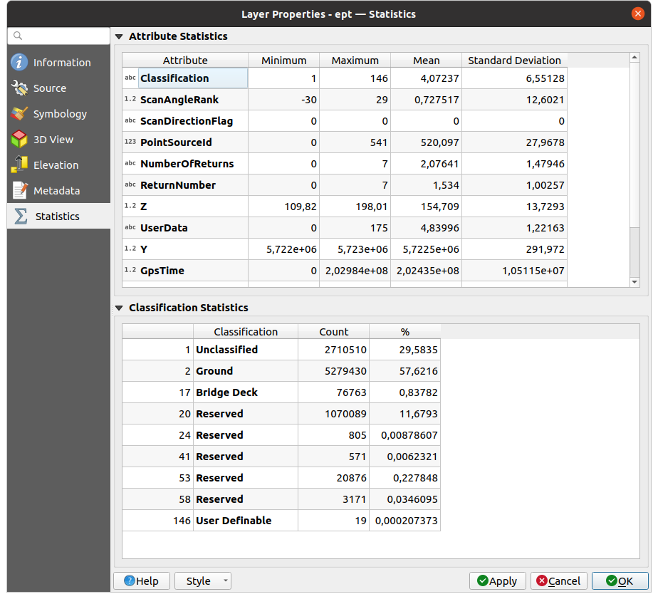
Fig. 20.10 De puntenwolk tab Statistieken