18. Travailler avec des données maillées (mesh)

18.1. Qu’est-ce qu’un maillage ?

Un maillage est une grille non structurée généralement avec des composants temporels et autres. La composante spatiale contient une collection de sommets, d’arêtes et de faces dans un espace 2D ou 3D.:

• sommets - points XY(Z) (dans le système de référence des coordonnées de la couche)

• arrêtes - connecte une paire de sommets

• faces : une face est définie par une série d’arêtes formant une surface fermée, typiquement un triangle ou un quadrilatère et, plus rarement, un polygone composé de plus de sommets

Sur la base de ce qui précède, les couches de maillage peuvent donc avoir différents types de structure :

• 1D Meshes: ils sont constitués de sommets et d’arêtes. Une arête relie deux sommets et peut recevoir des données (scalaires ou vectorielles). Le réseau maillé 1D peut par exemple être utilisé pour la modélisation d’un système de drainage urbain.

• 2D meshes: consistent en des faces avec des triangles, des quadrangles réguliers ou non structurés.

• 3D layered meshes: consistent en plusieurs maillages 2D non structurés empilés, chacun étant extrudé dans la direction verticale (niveaux) au moyen d’une coordonnée verticale. Les sommets et les faces ont la même topologie dans chaque niveau vertical. La définition du maillage (extrusion des niveaux verticaux) peut en général changer dans le temps. Les données sont généralement définies en centres de volume ou par une fonction paramétrique.

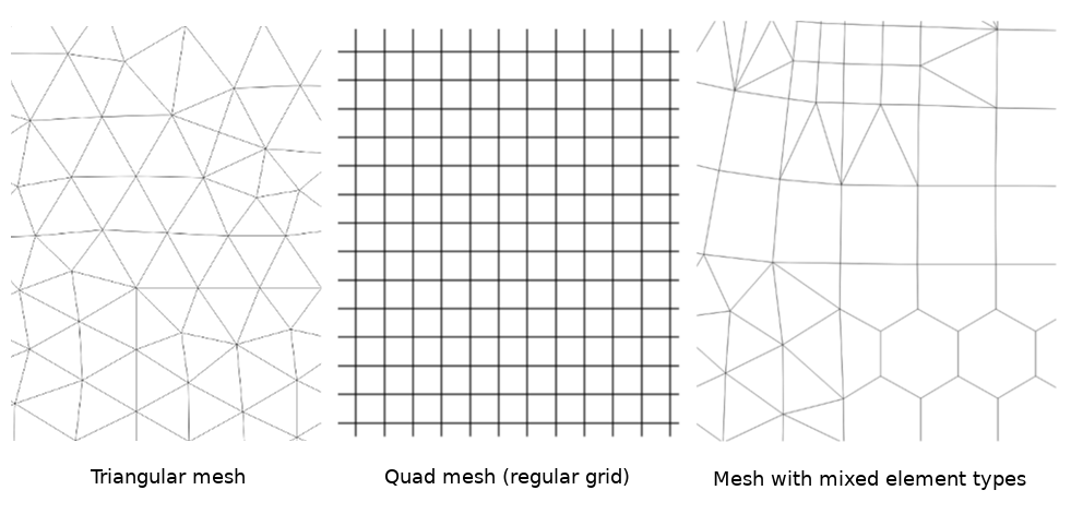
Fig. 18.1 Différents types de maillage

Le maillage fournit les information sur la structure spatiale. En plus, un maillage peut contenir des jeux de données (des groupes) qui attribuent une valeur à chaque sommet. Voici un exemple avec un maillage triangulaire dont les numéros de sommets apparaissent sur l’image ci-dessous :

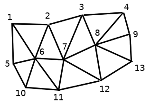
Fig. 18.2 Maillage triangulaire dont les sommets sont numérotés

Chaque sommet peut stocker plusieurs jeux de données (très souvent de grandes quantités) et ceux-ci peuvent avoir également une dimension temporelle. Ainsi, un unique fichier peut contenir de très nombreux jeux de données.

Le tableau qui suit donne une idée des informations qui peuvent être stockées dans les jeux de données maillés. Les colonnes correspondent aux numéros des sommets et chaque ligne représente un jeu de données. Les jeux de données peuvent être de différents types. Dans cet exemple, il s’agit de la vitesse du vent à 10m à différents moments (t1, t2, t3).

De la même manière, un jeu de données maillé peut stocker des vecteurs de valeurs pour chaque sommet. Par exemple, la direction du vent à un moment donné :

Tableau 18.1 Exemple de jeu de données de maillage

Vent à 10m	1	2	3	…
Vitesse à 10m au temps t1	17251	24918	32858	…
Vitesse à 10m au temps t2	19168	23001	36418	…
Vitesse à 10m au temps t3	21085	30668	17251	…
…	…	…	…	…
Direction du vent à 10m au temps t1	[20,2]	[20,3]	[20,4.5]	…
Direction du vent à 10m au temps t2	[21,3]	[21,4]	[21,5.5]	…
Direction du vent à 10m au temps t3	[22,4]	[22,5]	[22,6.5]	…
…	…	…	…	…

Nous pouvons visualiser les données en attribuant des couleurs aux valeurs (de la même façon que pour les rendus raster en Pseudo-couleur à bande unique) et en interpolant les données entre les sommets en fonction de la topologie. Il est courant que les valeurs soient des vecteurs 2D plutôt que de simples valeurs scalaires (comme pour la direction du vent). Pour de tels types de valeurs, il est préférable d’afficher des flèches indiquant les directions.

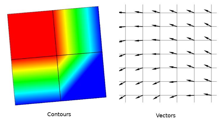
Fig. 18.3 Exemples de visualisation de données maillées

18.2. Formats de données gérés

QGIS accède aux données maillées à l’aide des drivers MDAL,et supporte nativement une variété de formats. La possibilité pour QGIS de modifier une couche de maillage dépend du format et du type de structure de maillage.

Pour charger un jeu de données maillé dans QGIS, utilisez la commande Maillage dans la boîte de dialogue Gestionnaire source de données. Lisez Chargement d’une couche de maillage pour plus de détails.

18.3. Propriétés d’un jeu de données maillé

The Layer Properties dialog for a mesh layer provides general settings to manage dataset groups of the layer and their rendering (active dataset groups, symbology, 2D and 3D rendering). It also provides information about the layer.

Pour ouvrir la fenêtre Propriétés de la couche :

• Dans le panneau Couches, effectuez un double-clic ou un clic droit et sélectionner Propriétés de la couche depuis le menu contextuel.

• Allez dans menu Couche ► Propriétés couche … lorsque la couche est sélectionnée.

The mesh Layer Properties dialog provides the following sections:

Tableau 18.2 Onglets des propriétés de la couche de maillage

Information	Source	Symbologie[1]
Vue 3D[1]	Temporel	Elevation
Rendu	Métadonnées

^[1] Aussi disponible dans le panneau Style de Couche

Note

Most of the properties of a mesh layer can be saved to or loaded from a .qml using the Style menu at the bottom of the dialog. More details at Gestion des styles personnalisés.

18.3.1. Onglet Information

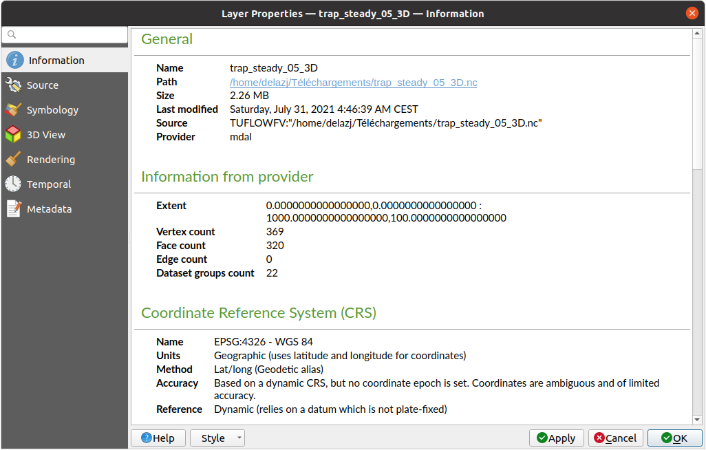
Fig. 18.4 Mesh Layer Information Properties

L’onglet Information, en lecture seule, permet d’avoir rapidement un résumé des informations et métadonnées de la couche courante. Les informations fournies sont :

• general such as name in the project, source path, list of auxiliary files, last save time and size, the used provider

• based on the provider of the layer: extent, vertex, face, edges and/or dataset groups count

• the Coordinate Reference System: name, units, method, accuracy, reference (i.e. whether it’s static or dynamic)

• extracted from filled metadata: access, extents, links, contacts, history…

18.3.2. Onglet Source

The Source tab displays basic information about the selected mesh, including:

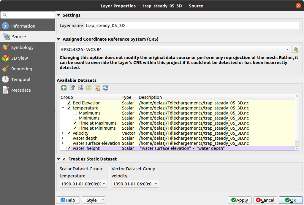
Fig. 18.5 Propriétés source de la couche de maillage

• the layer name to display in the Layers panel

• setting the Coordinate Reference System: Displays the layer’s Assigned Coordinate Reference System (CRS). You can change the layer’s CRS by selecting a recently used one in the drop-down list or clicking on Select CRS button (see Sélectionneur de Système de Coordonnées de Référence). Use this process only if the CRS applied to the layer is wrong or if none was applied.

• The Available datasets frame lists all the dataset groups (and subgroups) in the mesh layer, with their type and description in a tree view. Both regular datasets (i.e. their data is stored in the file) and virtual datasets (which are calculated on the fly) are listed.

  • Use the Assign extra dataset to mesh button to add more groups to the current mesh layer.

  • Collapse all and Expand all the dataset tree, in case of embedded groups

  • Si vous n’êtes intéressé que par certain jeux de données, vous pouvez décocher les autres et les rendre indisponibles dans le projet

  • Double-cliquez sur un nom et vous pouvez renommer le jeu de données.

  • Reset to defaults: checks all the groups and renames them back to their original name in the provider.

  • Right-click over a virtual dataset group and you can:

    • Remove dataset group from the project

    • Save dataset group as… a file on disk, to any supported format. The new file is kept assigned to the current mesh layer in the project.

• Checking the Treat as static dataset group allows to ignore the map temporal navigation properties while rendering the mesh layer. For each active dataset group (as selected in Symbology ► Datasets tab), you can:

  • set to None: the dataset group is not displayed at all

  • Display dataset: e.g., for the « bed elevation » dataset which is not time aware

  • extract a particular date time: the dataset matching the provided time is rendered and stay fixed during map navigation.

18.3.3. Onglet Style

Click the Symbology button to activate the dialog. Symbology properties are divided into several tabs:

• Datasets

• Contours

• Vectors

• Rendering

• Stacked mesh averaging method

18.3.3.1. Datasets

The tab ^Datasets is the main place to control and set which datasets will be used for the layer. It presents the following items:

• Groups available in the mesh dataset, with whether they provide:

  • scalar dataset

  • or vector dataset: by default, each vector dataset has a scalar dataset representing its magnitude automatically generated.

  Click on the icon next to the dataset name to select the group and type of data to represent.

• Selected dataset group(s) metadata, with details on:

  • the mesh type: edges or faces

  • the data type: vertices, edges, faces or volume

  • whether it’s of vector type or not

  • the original name in the mesh layer

  • the unit, if applicable

• blending mode available for the selected datasets.

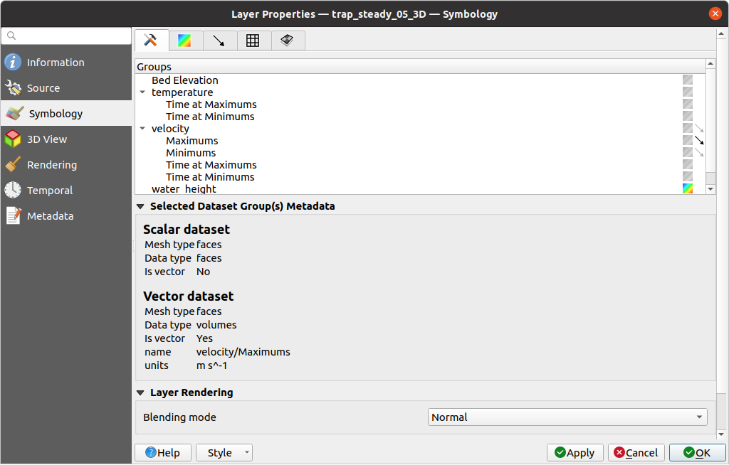
Fig. 18.6 Mesh Layer Datasets

You can apply symbology to the selected vector and/or scalar group using the next tabs.

18.3.3.2. Symbologie des contours

Note

The ^Contours tab can be activated only if a scalar dataset has been selected in the Datasets tab.

In the ^Contours tab you can see and change the current visualization options of contours for the selected group, as shown in Fig. 18.7 below:

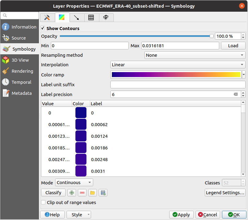
Fig. 18.7 Styliser les contours dans une couche maillée

• For 1D mesh, set the Stroke width of the edges. This can be a fixed size for the whole dataset, or vary along the geometry (more details with the interpolated line renderer)

• Use the slider or the spinbox to set the Opacity of the current group, if of a 2D mesh type.

• Enter the range of values you want to represent on the current group: use ^Load to fetch the min and max values of the current group or enter custom values if you want to exclude some.

• For 2D/3D meshes, select the Resampling method to interpolate the values on the surrounding vertices to the faces (or from the surrounding faces to the vertices) using the Neighbour average method. Depending on whether the dataset is defined on the vertices (respectively on the faces), QGIS defaults this setting to None (respectively Neighbour average) method in order to use values on vertices and keep the default rendering smooth.

• Classify the dataset using the color ramp shader classification.

18.3.3.3. Symbologie des vecteurs

Note

The ^Vectors tab can be activated only if a vector dataset has been selected in the Datasets tab.

In the ^Vectors tab you can see and change the current visualization options of vectors for the selected group, as shown in Fig. 18.8:

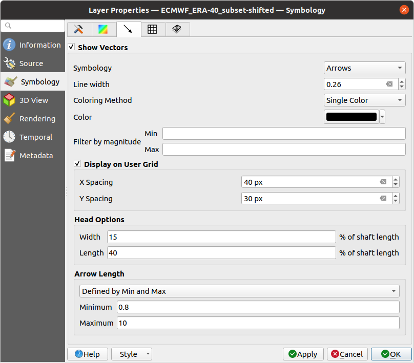
Fig. 18.8 Styling Vectors in a Mesh Layer with arrows

Mesh vector dataset can be styled using various types of Symbology:

• Arrows: vectors are represented with arrows at the same place as they are defined in the raw dataset (i.e. on the nodes or center of elements) or on a user-defined grid (hence, they are evenly distributed). The arrow length is proportional to the magnitude of the arrow as defined in the raw data but can be scaled by various methods.

• Streamlines: vectors are represented with streamlines seeded from start points. The seeding points can start from the vertices of the mesh, from a user grid or randomly.

• Traces: a nicer animation of the streamlines, the kind of effect you get when you randomly throws sand in the water and see where the sand items flows.

Available properties depend on the selected symbology as shown in the following table.

Tableau 18.3 Availability and meaning of the vectors symbology properties

Label	Description and Properties	Arrow	Streamlines	Traces
Line width	Width of the vector representation
Coloring method	a Single color assigned to all vectors or a variable color based on vectors magnitude, using a Color ramp shader
Filter by magnitude	Only vectors whose length for the selected dataset falls between a Min and Max range are displayed
Display on user grid	Places the vector on a grid with custom X spacing and Y spacing and interpolates their length based on neighbours
Head options	Length and Width of the arrow head, as a percentage of its shaft length
Arrow length	Defined by Min and Max: You specify the minimum and maximum length for the arrows, QGIS will interpolate their size based on the underlying vector’s magnitude Scale to magnitude: arrow length is proportional to their vector’s magnitude Fixed: all the vectors are shown with the same length
Streamlines seeding method	On mesh/grid: relies on the user grid to display the vectors Randomly: vector placement is randomly done with respect to a certain density
Particles count	The amount of « sand » you want to throw into visualisation
Max tail length	The time until the particle fades out

18.3.3.4. Rendu

In the tab ^Rendering tab, QGIS offers possibilities to display and customize the mesh structure. Line width and Line color can be set to represent:

• the edges for 1D meshes

• For 2D meshes:

  • Native mesh rendering: shows original faces and edges from the layer

  • Triangular mesh rendering: adds more edges and displays the faces as triangles

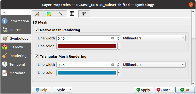
Fig. 18.9 2D Mesh Rendering

18.3.3.5. Stacked mesh averaging method

3D layered meshes consist of multiple stacked 2D unstructured meshes each extruded in the vertical direction (levels) by means of a vertical coordinate. The vertices and faces have the same topology in each vertical level. Values are usually stored on the volumes that are regularly stacked over base 2d mesh. In order to visualise them on 2D canvas, you need to convert values on volumes (3d) to values on faces (2d) that can be shown in mesh layer. The ^{Stacked mesh averaging method} provides different averaging/interpolation methods to handle this.

You can select the method to derive the 2D datasets and corresponding parameters (level index, depth or height values). For each method, an example of application is shown in the dialog but you can read more on the methods at https://fvwiki.tuflow.com/index.php?title=Depth_Averaging_Results.

18.3.4. Propriétés de la vue 3D

Mesh layers can be used as terrain in a 3D map view based on their vertices Z values. From the 3D View properties tab, it’s also possible to render the mesh layer’s dataset in the same 3D view. Therefore, the vertical component of the vertices can be set equal to dataset values (for example, level of water surface) and the texture of the mesh can be set to render other dataset values with color shading (for example velocity).

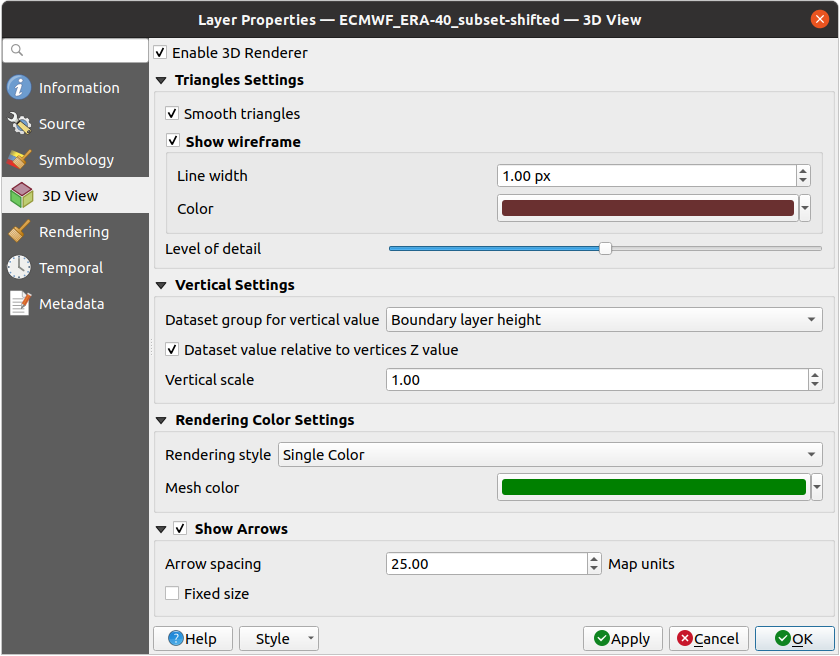
Fig. 18.10 Mesh dataset 3D properties

Check Enable 3D Renderer and you can edit following properties:

• Under Triangle settings

  • Smooth triangles: Angles between consecutive triangles are smoothed for a better 3D rendering

  • Show wireframe whose you can set the Line width and Color

  • Level of detail: Controls how simplified the mesh layer to render should be. On the far right, it is the base mesh, and the more you go left, the more the layer is simplified and is rendered with less details. This option is only available if the Simplify mesh option under the Rendering tab is activated.

• Vertical settings to control behavior of the vertical component

  of vertices of rendered triangles

  • Dataset group for vertical value: the dataset group that will be used for the vertical component of the mesh

  • Dataset value relative to vertices Z value: whether to consider the dataset values as absolute Z coordinate or relative to the vertices native Z value

  • Vertical scale: the scale factor to apply to the dataset Z values

• Rendering color settings with a Rendering style that can be based on the color ramp shader set in Symbologie des contours (2D contour color ramp shader) or as a Single color with an associated Mesh color

• Show arrows: displays arrows on mesh layer dataset 3D entity, based on the same vector dataset group used in the vector 2D rendering. They are displayed using the 2D color setting. It’s also possible to define the Arrow spacing and, if it’s of a Fixed size or scaled on magnitude. This spacing setting defines also the max size of arrows because arrows can’t overlap.

18.3.5. Onglet Rendu

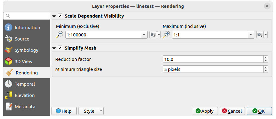
Fig. 18.11 Mesh rendering properties

Under the Scale dependent visibility group box, you can set the Maximum (inclusive) and Minimum (exclusive) scale, defining a range of scale in which mesh elements will be visible. Out of this range, they are hidden. The ^{Set to current canvas scale} button helps you use the current map canvas scale as boundary of the range visibility. See Sélecteur de visibilité définie par l’échelle for more information.

Note

Vous pouvez aussi activer l’échelle de visibilité sur une couche depuis le panneau de couches. Clic-droit sur la couche et dans le menu contextuel, sélectionner Définir l’échelle de visibilité.

As mesh layers can have millions of faces, their rendering can sometimes be very slow, especially when all the faces are displayed in the view whereas they are too small to be viewed. To speed up the rendering, you can simplify the mesh layer, resulting in one or more meshes representing different levels of detail and select at which level of detail you would like QGIS to render the mesh layer. Note that the simplify mesh contains only triangular faces.

From the Rendering tab, check Simplify mesh and set:

• a Reduction factor: Controls generation of successive levels of simplified meshes. For example, if the base mesh has 5M faces, and the reduction factor is 10, the first simplified mesh will have approximately 500 000 faces, the second 50 000 faces, the third 5000,… If a higher reduction factor leads quickly to simpler meshes (i.e. with triangles of bigger size), it produces also fewer levels of detail.

• Minimum triangle size: the average size (in pixels) of the triangles that is permitted to display. If the average size of the mesh is lesser than this value, the rendering of a lower level of details mesh is triggered.

18.3.6. Propriétés temporelles

The Temporal tab provides options to control the rendering of the layer over time. It allows to dynamically display temporal values of the enabled dataset groups. Such a dynamic rendering requires the temporal navigation to be enabled over the map canvas.

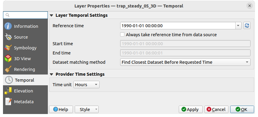
Fig. 18.12 Mesh Temporal properties

Layer temporal settings

• Reference time of the dataset group, as an absolute date time. By default, QGIS parses the source layer and returns the first valid reference time in the layer’s dataset group. If unavailable, the value will be set by the project time range or fall back to the current date. The Start time and End time to consider are then calculated based on the internal timestamp step of the dataset.

  It is possible to set a custom Reference time (and then the time range), and revert the changes using the ^{Reload from provider} button. With Always take reference time from data source checked, you ensure that the time properties are updated from the file each time the layer is reloaded or the project reopened.

• Dataset matching method: determines the dataset to display at the given time. Options are Find closest dataset before requested time or Find closest dataset from requested time (after or before).

Provider time settings

• Time unit extracted from the raw data, or user defined. This can be used to align the speed of the mesh layer with other layers in the project during map time navigation. Supported units are Seconds, Minutes, Hours and Days.

18.3.7. Onglet Élévation

The Elevation tab provides options to control the layer elevation properties within a 3D map view and its appearance in the profile tool charts. Specifically, you can set:

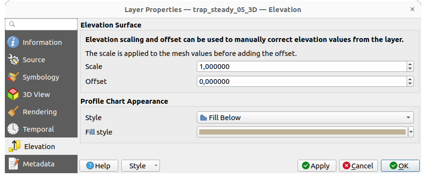
Fig. 18.13 Mesh Elevation properties

• Elevation Surface: how the mesh layer vertices Z values should be interpreted as terrain elevation. You can apply a Scale factor and an Offset.

• Profile Chart Appearance: controls the rendering Style the mesh elevation will use when drawing a profile chart. It can be set as:

  • a profile Line with a line style applied

  • a surface with Fill below and a corresponding fill style

18.3.8. Onglet Métadonnées

L’onglet Métadonnées vous offre des options pour créer et modifier un rapport de métadonnées sur votre couche. Voir Metadata pour plus d’informations.

18.4. Editing a mesh layer

QGIS allows to create a mesh layer from scratch or based on an existing one. You can create/modify the geometries of the new layer whom you can assign datasets afterwards. It’s also possible to edit an existing mesh layer. Because the editing operation requires a frames-only layer, you will be asked to either remove any associated datasets first (make sure you have them available if they still are necessary) or create a copy (only geometries) of the layer.

Note

QGIS does not allow to digitize edges on mesh layers. Only vertices and faces are mesh elements that can be created. Also not all supported mesh formats can be edited in QGIS (see permissions).

18.4.1. Overview of the mesh digitizing tools

To interact with or edit a base mesh layer element, following tools are available.

Tableau 18.4 Tools for mesh digitizing

Label	Fonction	Location
Current Edits	Access to save, rollback or cancel changes in all or selected layers simultaneously	Digitizing toolbar
Toggle to Edit	Turn on/off the layer in edit mode	Digitizing toolbar
Save Edits	Save changes done to the layer	Digitizing toolbar
Undo	Undo the last change(s) - Ctrl+Z	Digitizing toolbar
Redo	Redo the last undone action(s) - Ctrl+Shift+Z	Digitizing toolbar
Enable Advanced Digitizing tools	Turn on/off the Advanced Digitizing Panel	Advanced Digitizing toolbar
Reindex Faces and Vertices	Recreate index and renumber the mesh elements for optimization	Mesh menu
Digitize Mesh Elements	Select/Create vertices and faces	Mesh Digitizing toolbar
Select Mesh Elements by Polygon	Select vertices and faces overlapped by a drawn polygon	Mesh Digitizing toolbar
Select Mesh Elements by Expression	Select vertices and faces using an expression	Mesh Digitizing toolbar
Transformer les coordonnées des sommets	Modify coordinates of a selection of vertices	Mesh Digitizing toolbar
Force by Selected Geometries	Split faces and constrain Z value using a linear geometry	Mesh Digitizing toolbar

18.4.2. Exploring the Z value assignment logic

When a mesh layer is turned into edit mode, a Vertex Z value widget opens at the top right of the map canvas. By default, its value corresponds to the Default Z value set in Settings ► Options ► Digitizing tab. When there are selected vertices, the widget displays the average Z value of the selected vertices.

During editing, the Vertex Z value is assigned to new vertices. It is also possible to set a custom value: edit the widget, press Enter and you will override the default value and make use of this new value in the digitizing process. Click the icon in the widget to reset its value to the Options default value.

18.4.2.1. Rules of assignment

When creating a new vertex, its Z value definition may vary depending on the active selection in the mesh layer and its location. The following table displays the various combinations.

Tableau 18.5 Matrix of Z value assignment to new vertex

Vertex creation	Are there selected vertices in mesh layer?	Source of assigned value	Assigned Z Value
« Free » vertex, not connected to any face or edge of a face	Non	Vertex Z value	Default or user defined
		Advanced Digitizing Panel (if z widget is in Locked state)	z widget if in Locked state
	Oui	Vertex Z value	Average of the selected vertices
Vertex on an edge	—	Mesh layer	Interpolated from the edge’s vertices
Vertex on a face	—	Mesh layer	Interpolated from the face’s vertices
Vertex snapped to a 2D vector feature	—	Vertex Z value	Default or user defined
Vertex snapped to a 3D vector vertex	—	Vector layer	Vertex
Vertex snapped to a 3D vector segment	—	Vector layer	Interpolated along the vector segment

Note

The Vertex Z value widget is deactivated if the Advanced Digitizing Panel is enabled and no mesh element is selected. The latter’s z widget then rules the Z value assignment.

18.4.2.2. Modifying Z value of existing vertices

To modify the Z value of vertices, the most straightforward way is:

1. Select one or many vertices. The Vertex Z value widget will display the average height of the selection.

2. Change the value in the widget.

3. Press Enter. The entered value is assigned to the vertices and becomes the default value of next vertices.

Another way to change the Z value of a vertex is to move and snap it on a vector layer feature with the Z value capability. If more than one vertex are selected, the Z value can’t be changed in this way.

The Transform mesh vertices dialog also provides means to modify the Z value of a selection of vertices (along with their X or Y coordinates).

18.4.3. Selecting mesh elements

18.4.3.1. Using Digitize Mesh Elements

Activate the ^{Digitize Mesh Elements} tool. Hover over an element and it gets highlighted, allowing you to select it.

• Click on a vertex, and it is selected.

• Click on the small square at the center of a face or an edge, and it gets selected. Connected vertices are also selected. Conversely, selecting all the vertices of an edge or a face also selects that element.

• Drag a rectangle to select overlapping elements (a selected face comes with all their vertices). Press Alt key if you want to select only completely contained elements.

• To add elements to a selection, press Shift while selecting them.

• To remove an element from the selection, press Ctrl and reselect it. A deselected face will also deselect all their vertices.

18.4.3.2. Using Select Mesh Elements by Polygon

Activate the ^{Select Mesh Elements by Polygon} tool and:

• Draw a polygon (left-click to add vertex, Backspace to undo last vertex, Esc to abort the polygon and right-click to validate it) over the mesh geometries. Any partially overlapping vertices and faces will get selected. Press Alt key while drawing if you want to select only completely contained elements.

• Right-click over the geometry of a vector layer’s feature, select it in the list that pops up and any partially overlapping vertices and faces of the mesh layer will get selected. Use Alt while drawing to select only completely contained elements.

• To add elements to a selection, press Shift while selecting them.

• To remove an element from the selection, press Ctrl while drawing over the selection polygon.

18.4.3.3. Using Select Mesh Elements by Expression

Another tool for mesh elements selection is ^{Select Mesh Elements by Expression}. When pressed, the tool opens the mesh expression selector dialog from which you can:

1. Select the method of selection:

   • Select by vertices: applies the entered expression to vertices, and returns matching ones and their eventually associated edges/faces

   • Select by faces: applies the entered expression to faces, and returns matching ones and their associated edges/vertices

2. Write the expression of selection. Depending on the selected method, available functions in the Meshes group will be filtered accordingly.

3. Run the query by setting how the selection should behave and pressing:

   • Select: replaces any existing selection in the layer

   • Add to current selection

   • Remove from current selection

18.4.4. Modifying mesh elements

18.4.4.1. Adding vertices

To add vertices to a mesh layer:

1. Press the ^{Digitize mesh elements} button

2. A Vertex Z value widget appears on the top right corner of the map canvas. Set this value to the Z coordinate you would like to assign to the subsequent vertices

3. Then double-click:

   • outside a face: adds a « free vertex », that is a vertex not linked to any face. This vertex is represented by a red dot when the layer is in editing mode.

   • on the edge of existing face(s): adds a vertex on the edge, splits the touching face(s) into triangles connected to the new vertex.

   • inside a face: splits the face into triangles whose edges connect the surrounding vertices to the new vertex.

18.4.4.2. Adding faces

To add faces to a mesh layer:

1. Press the ^{Digitize mesh elements} button

2. A Vertex Z value widget appears on the top right corner of the map canvas. Set this value to the Z coordinate you would like to assign to the subsequent vertices.

3. Hover over a vertex and click the small triangle that appears next it.

4. Move the cursor to the next vertex position; you can snap to existing vertex or left-click to add a new one.

5. Proceed as above to add as many vertices you wish for the face. Press Backspace button to undo the last vertex.

6. While moving the mouse, a rubberband showing the shape of the face is displayed. If it is shown in green, then the expected face is valid and you can right-click to add it to the mesh. If it is red, the face is not valid (e.g. because it self-intersects, overlaps an existing face or vertex, creates a hole, …) and can’t be added. You’d need to undo some vertices and fix the geometry.

7. Press Esc to abort the face digitizing.

8. Right-click to validate the face.

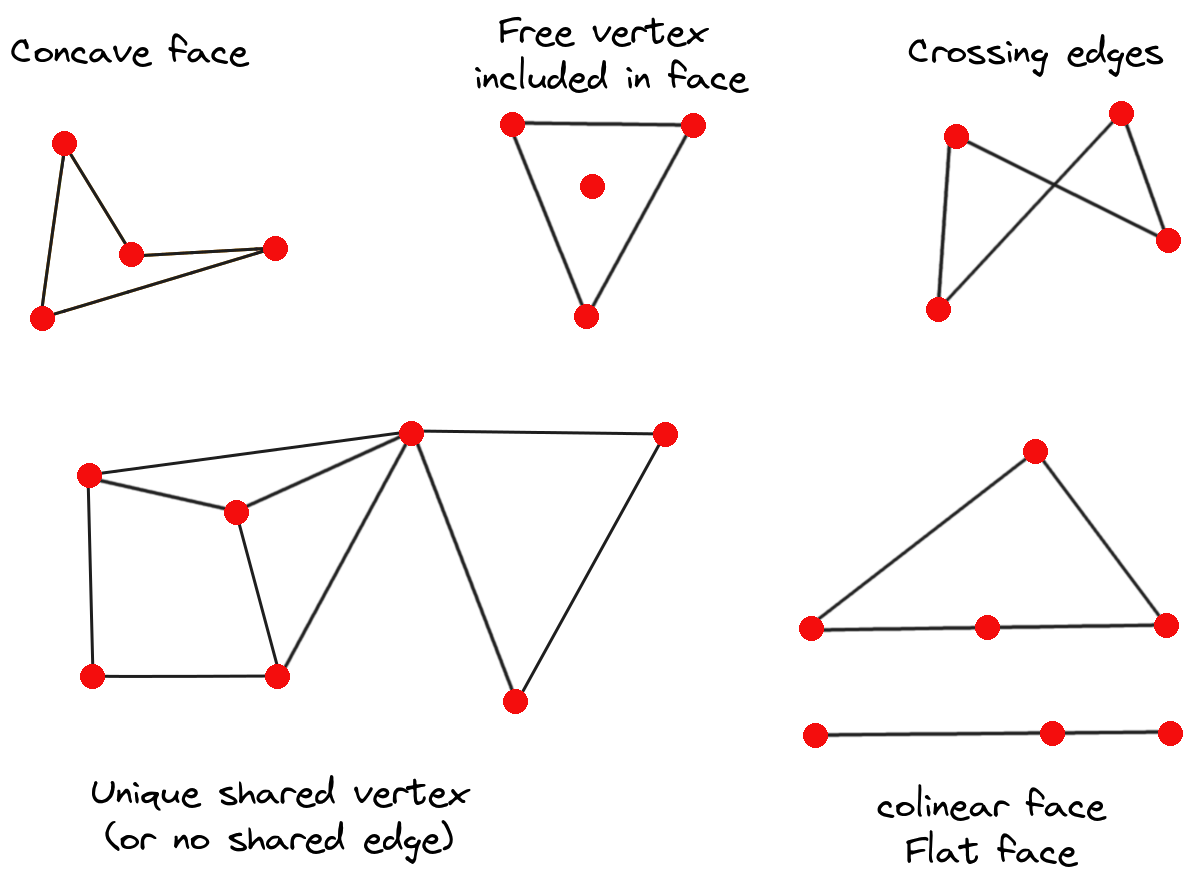
Fig. 18.14 Examples of invalid mesh

18.4.4.3. Removing mesh elements

1. Select the target elements

2. Enable the ^{Digitize mesh elements} tool

3. Right-click and select:

   • Remove Selected Vertices and Fill Hole(s) or press Ctrl+Del: removes vertices and linked faces and fills the hole(s) by triangulating from the neighbor vertices

   • Remove Selected Vertices Without Filling Hole(s) or press Ctrl+Shift+Del: removes vertices and linked faces and do not fill hole(s)

   • Remove Selected Face(s) or press Shift+Del: removes faces but keeps the vertices

These options are also accessible from the contextual menu when hovering over a single item without selecting.

18.4.4.4. Moving mesh elements

To move vertices and faces of a mesh layer:

1. Select the target elements

2. Enable the ^{Digitize mesh elements} tool

3. To start moving the element, click on a vertex or the centroid of a face/edge

4. Move the cursor to the target location (snapping to vector features is supported).

5. If the new location does not generate an invalid mesh, the moved elements appear in green. Click again to release them at this location. Faces whose vertices are all selected are translated, their neighbors are reshaped accordingly.

18.4.4.5. Transforming mesh vertices

The ^{Transform Vertices Coordinates} tool gives a more advanced way to move vertices, by editing their X, Y and/or Z coordinates thanks to expressions.

1. Select the vertices you want to edit the coordinates

2. Press ^{Transform Vertices Coordinates}. A dialog opens with a mention of the number of selected vertices. You can still add or remove vertices from the selection.

3. Depending on the properties you want to modify, you need to check the X coordinate, Y coordinate and/or Z value.

4. Then enter the target position in the box, either as a numeric value or an expression (using the ^{Expression dialog})

5. With the ^{Import Coordinates of the Selected Vertex} pressed, the X, Y and Z boxes are automatically filled with its coordinates whenever a single vertex is selected. A convenient and quick way to adjust vertices individually.

6. Press Preview Transform to simulate the vertices new location and preview the mesh with transformation.

   • If the preview is green, transformed mesh is valid and you can apply the transformation.

   • If the preview is red, the transformed mesh is invalid and you can not apply the transformation until it is corrected.

7. Press Apply Transform to modify the selected coordinates for the set of vertices.

18.4.4.6. Reshaping mesh geometry

The contextual menu

1. Enable the ^{Digitize mesh elements}

2. Select mesh item(s), or not

3. Hover over a mesh element, it gets highlighted.

4. Right-click and you can:

   • remove the item(s)

   • Split Selected Face(s) (Split Current Face): splits the face you are hovering over or each selected quad mesh faces into two triangles

   • Delaunay Triangulation with Selected vertices: builds triangular faces using selected free vertices.

   • Refine Selected Face(s) (Refine Current Face): splits the face into four faces, based on vertices added at the middle of each edge (a triangle results into triangles, a quad into quads). Also triangulates adjacent faces connected to the new vertices.

The edge markers

When the ^{Digitize mesh elements} is active and you hover over an edge, the edge is highlighted and it is possible to interact with it. Depending on the context, following markers may be available:

• a square, at the center of the edge: click on it to select extremity vertices.

• a cross if the two faces on either side can be merged: click on it to delete the edge and merge the faces.

• a circle if the edge is between two triangles: Click on it to flip the edge, i.e. connect it instead to the two other « free » vertices of the faces

The Force by Selected Geometries tool

The ^{Force by Selected Geometries} tool provides advanced ways to apply break lines using lines geometry. A break line will force the mesh to have edges along the line. Note that the break line will not be considered persistent once the operation is done; resulting edges will not act as constraints anymore and can be modified like any other edge. This can be used for example to locally modify a mesh layer with accurate lines, as river banks or border of road embankments.

1. Enable the ^{Force by Selected Geometries} tool

2. Indicate the geometry to use as « forcing line »; it can be:

   • picked from a line or polygon feature in the map canvas: right-click over the vector feature and select it from the list in the contextual menu.

   • a virtual line drawn over the mesh frame: left-click to add vertices, right-click for validation. Vertices Z value is set through the Vertex Z value widget or the z widget if the Advanced Digitizing Panel is on. If the line is snapped to a mesh vertex or a 3D vector feature’s vertex or segment, the new vertex takes the snapped element Z value.

Mesh faces that overlap the line geometry or the polygon’s boundary will be affected in a way that depends on options you can set from the ^{Force by Selected Geometries} tool drop-down menu:

• Add new vertex on intersecting edges: with this option, a new vertex is added each time the forcing line intersect an edge. This option leads to split along the line each encountered faces.

  Without this option, encountered faces are removed and replaced by faces coming from a triangulation with only the existing vertices plus the vertices of the forcing lines (new vertices are also added on the boundary edge intersecting the forcing lines).

  

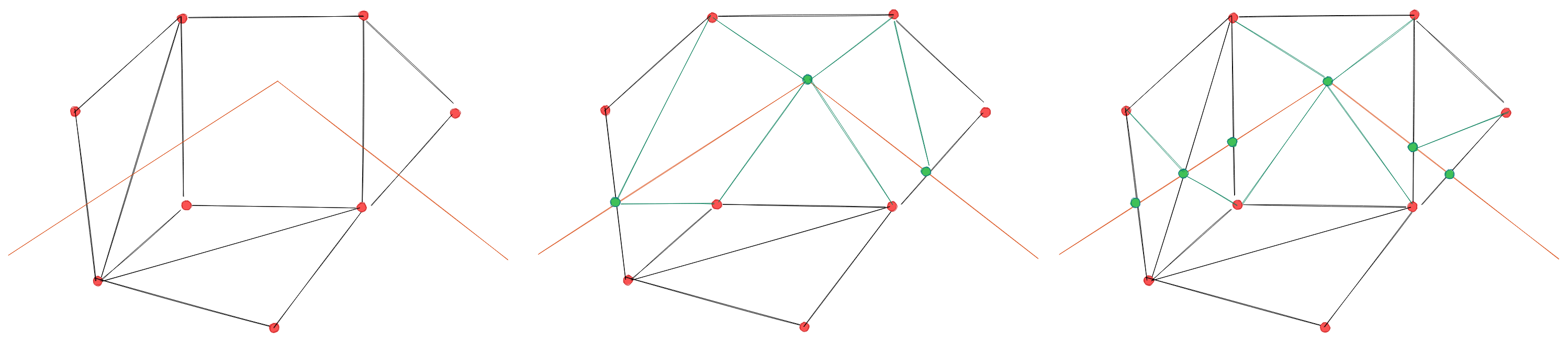
  Fig. 18.15 Force Mesh using a line geometry - Results without (middle) and with (right) new vertex on edges intersection

• Interpolate Z value from: set how the new vertices Z value is calculated. It can be from:

  • the Mesh itself: the new vertices Z value is interpolated from vertices of the face they fall within

  • or the Forcing line: if the line is defined by a 3D vector feature or a drawn line then the new vertices Z value is derived from its geometry. In case of 2D line feature, the new vertices Z value is the Vertex Z value.

• Tolerance: when an existing mesh vertex is closer to the line than the tolerance value, do not create new vertex on the line but use the existing vertex instead. The value can be set in Meters at Scale or in Map Units (more details at Sélecteur d’unité).

18.4.5. Reindexing meshes

During edit, and in order to allow quick undo/redo operations, QGIS keeps empty places for deleted elements, which may lead to growing memory use and inefficient mesh structuring. The Mesh ► Reindex Faces and Vertices tool is designed to remove these holes and renumber the indices of faces and vertices so that they are continuous and somewhat reasonably ordered. This optimizes relation between faces and vertices and increases the efficiency of calculation.

Note

The Reindex Faces and Vertices tool saves the layer and clear the undo/redo stacks, disabling any rollback.

18.5. Mesh Calculator

The Mesh Calculator tool from the top Mesh menu allows you to perform arithmetic and logical calculations on existing dataset groups to generate a new dataset group (see Fig. 18.16).

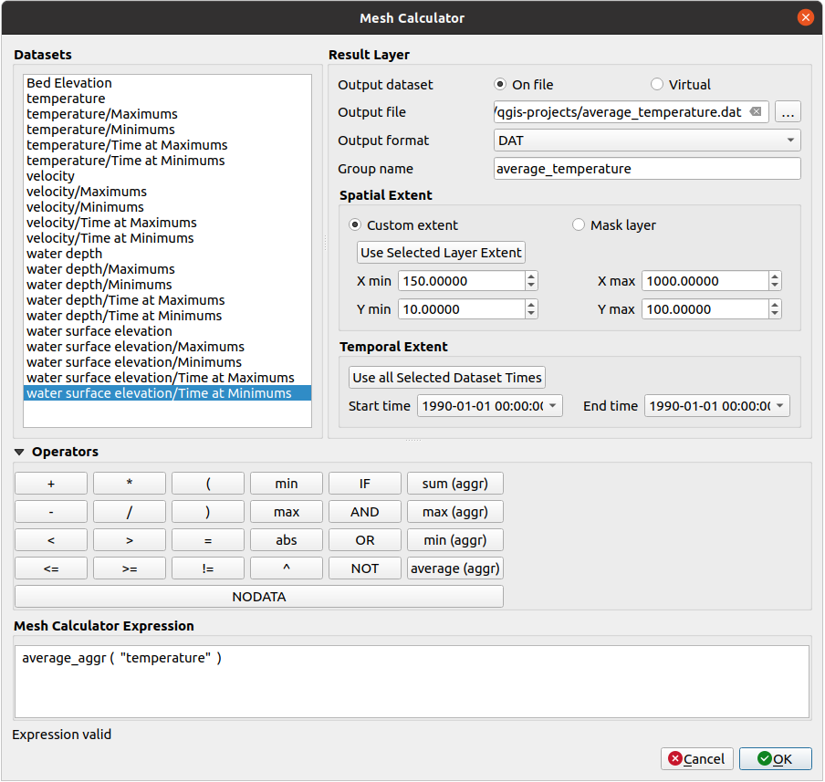
Fig. 18.16 Mesh Calculator

The Datasets list contains all dataset groups in the active mesh layer. To use a dataset group in an expression, double click its name in the list and it will be added to the Mesh calculator expression field. You can then use the operators to construct calculation expressions, or you can just type them into the box.

The Result Layer helps you configure properties of the output layer:

• Create on-the-fly dataset group instead of writing layer to disk:

  • If unchecked, the output is stored on disk as a new plain file. An Output File path and an Output Format are required.

  • If checked, a new dataset group will be added to the mesh layer. Values of the dataset group are not stored in memory but each dataset is calculated when needed with the formula entered in the mesh calculator. That virtual dataset group is saved with the project, and if needed, it can be removed or made persistent in file from the layer Source properties tab.

  In either case, you should provide a Group Name for the output dataset group.

• The Spatial extent to consider for calculation can be:

  • a Custom extent, manually filled with the X min, X max, Y min and Y max coordinate, or extracted from an existing dataset group (select it in the list and press Use selected layer extent to fill the abovementioned coordinate fields)

  • defined by a polygon layer (Mask layer) of the project: the polygon features geometry are used to clip the mesh layer datasets

• The Temporal extent to take into account for datasets can be set with the Start time and End time options, selected from the existing dataset groups timesteps. They can also be filled using the Use all selected dataset times button to take the whole range.

The Operators section contains all available operators. To add an operator to the mesh calculator expression box, click the appropriate button. Mathematical calculations (+, -, *, … ) and statistical functions (min, max, sum (aggr), average (aggr), … ) are available. Conditional expressions (=, !=, <, >=, IF, AND, NOT, … ) return either 0 for false and 1 for true, and therefore can be used with other operators and functions. The NODATA value can also be used in the expressions.

The Mesh Calculator Expression widget shows and lets you edit the expression to execute.