11.1. Opening Data
As part of an Open Source Software ecosystem, QGIS is built upon different libraries that, combined with its own providers, offer capabilities to read and often write a lot of formats:
Vector data formats include GeoPackage, GML, GeoJSON, GPX, KML, Comma Separated Values, ESRI formats (Shapefile, Geodatabase…), MapInfo and MicroStation file formats, AutoCAD DWG/DXF, GRASS and many more… Read the complete list of supported vector formats.
Raster data formats include GeoTIFF, JPEG, ASCII Gridded XYZ, MBTiles, R or Idrisi rasters, GDAL Virtual, SRTM, Sentinel Data, ERDAS IMAGINE, ArcInfo Binary Grid, ArcInfo ASCII Grid, and many more… Read the complete list of supported raster formats.
Database formats include PostgreSQL, SQLite/SpatiaLite, Oracle, MS SQL Server, SAP HANA, MySQL…
Web map and data services (WM(T)S, WFS, WCS, CSW, XYZ tiles, ArcGIS services, …) are also handled by QGIS providers. See Working with OGC / ISO protocols for more information about some of these.
You can read supported files from archived folders and use QGIS native formats such as QML files (QML - The QGIS Style File Format) and virtual and memory layers.
More than 80 vector and 140 raster formats are supported by GDAL and QGIS native providers.
Note
Not all of the listed formats may work in QGIS for various reasons.
For example, some require external proprietary libraries, or the GDAL/OGR
installation of your OS may not have been built to support the format you
want to use. To see the list of available formats, run the command line
ogrinfo --formats (for vector) and gdalinfo --formats (for raster),
or check the menu in QGIS.
In QGIS, depending on the data format, there are different tools to open a
dataset, mainly available in the menu
or from the Manage Layers toolbar (enabled through
menu).
However, all these tools point to a unique dialog, the Data Source
Manager dialog, that you can open with the  Open Data Source Manager button, available on the Data Source
Manager Toolbar, or by pressing Ctrl+L.
The Data Source Manager dialog (Fig. 11.1)
offers a unified interface to open file-based data as well as databases or
web services supported by QGIS.
Open Data Source Manager button, available on the Data Source
Manager Toolbar, or by pressing Ctrl+L.
The Data Source Manager dialog (Fig. 11.1)
offers a unified interface to open file-based data as well as databases or
web services supported by QGIS.
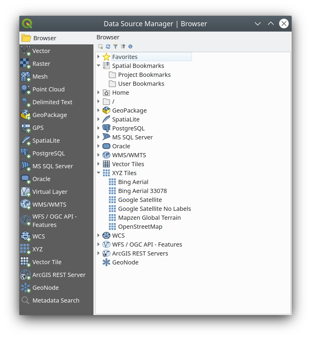
Fig. 11.1 QGIS Data Source Manager dialog
Beside this main entry point, you also have the  DB Manager plugin that offers advanced capabilities to analyze and
manipulate connected databases.
More information on DB Manager capabilities can be found in DB Manager Plugin.
DB Manager plugin that offers advanced capabilities to analyze and
manipulate connected databases.
More information on DB Manager capabilities can be found in DB Manager Plugin.
There are many other tools, native or third-party plugins, that help you open various data formats.
This chapter will describe only the tools provided by default in QGIS for loading data. It will mainly focus on the Data Source Manager dialog but more than describing each tab, it will also explore the tools based on the data provider or format specificities.
11.1.1. The Browser Panel
The Browser is one of the main ways to quickly and easily add your data to projects. It’s available as:
a Data Source Manager tab, enabled pressing the
Open Data Source Manager button (Ctrl+L);as a QGIS panel you can open from the menu (or
 ) or by pressing Ctrl+2.
In both cases, the Browser helps you navigate in your file system and manage geodata, regardless the type of layer (raster, vector, table), or the datasource format (plain or compressed files, databases, web services).
11.1.1.1. Exploring the Interface
At the top of the Browser panel, you find some buttons that help you to:
 Add Selected Layers: you can also add data to the map
canvas by selecting Add selected layer(s) from the layer’s context menu;
Add Selected Layers: you can also add data to the map
canvas by selecting Add selected layer(s) from the layer’s context menu; Refresh the browser tree;
 Filter Browser to search for specific data. Enter a search
word or wildcard and the browser will filter the tree to only show paths to
matching DB tables, filenames or folders – other data or folders won’t be
displayed. See the Browser Panel(2) example in Fig. 11.2.
The comparison can be case-sensitive or not. It can also be set to:
Filter Browser to search for specific data. Enter a search
word or wildcard and the browser will filter the tree to only show paths to
matching DB tables, filenames or folders – other data or folders won’t be
displayed. See the Browser Panel(2) example in Fig. 11.2.
The comparison can be case-sensitive or not. It can also be set to:Normal: show items containing the search text
Wildcard(s): fine tune the search using the
?and/or*characters to specify the position of the search textRegular expression
 Collapse All the whole tree;
 Enable/disable properties widget: when toggled on,
a new widget is added at the bottom of the panel showing, if applicable,
metadata for the selected item.
Enable/disable properties widget: when toggled on,
a new widget is added at the bottom of the panel showing, if applicable,
metadata for the selected item.
The entries in the Browser panel are organised hierarchically, and there are several top level entries:
Favorites where you can place shortcuts to often used locations
Spatial Bookmarks where you can store often used map extents (see Bookmarking extents on the map)
Project Home: for a quick access to the folder in which (most of) the data related to your project are stored. The default value is the directory where your project file resides.
Home directory in the file system and the filesystem root directory.
Connected local or network drives
Then comes a number of container / database types and service protocols, depending on your platform and underlying libraries:
 GeoPackage
 SpatiaLite
 PostgreSQL
 SAP HANA
 MS SQL Server
 Oracle
 WMS/WMTS
 Vector Tiles
 XYZ Tiles
 WCS
WCS WFS/OGC API-Features
 ArcGIS REST Server
11.1.1.2. Interacting with the Browser items
The browser supports drag and drop within the browser, from the browser to the canvas and Layers panel, and from the Layers panel to layer containers (e.g. GeoPackage) in the browser.
Project file items inside the browser can be expanded, showing the full layer tree (including groups) contained within that project. Project items are treated the same way as any other item in the browser, so they can be dragged and dropped within the browser (for example to copy a layer item to a geopackage file) or added to the current project through drag and drop or double click.
The context menu for an element in the Browser panel is opened by right-clicking on it.
For file system directory entries, the context menu offers the following:
to create in the selected entry a:
Directory…
GeoPackage…
ShapeFile…
Add as a Favorite: favorite folders can be renamed (Rename favorite…) or removed (Remove favorite) any time.
Hide from Browser: hidden folders can be toggled to visible from the setting
Fast Scan this Directory
Open Directory
Open in Terminal
Properties…
Directory Properties…
For leaf entries that can act as layers in the project, the context menu will have supporting entries. For example, for non-database, non-service-based vector, raster and mesh data sources:
Add Layer to Project
Layer Properties
Open with Data Source Manager…
or Delete “<name of file>”…
Show in Files
File Properties
In the Layer properties entry, you will find (similar to what you will find in the vector and raster layer properties once the layers have been added to the project):
Metadata for the layer. Metadata groups: Information from provider (if possible, Path will be a hyperlink to the source), Identification, Extent, Access, Fields (for vector layers), Bands (for raster layers), Contacts, Links (for vector layers), References (for raster layers), History.
A Preview panel
The attribute table for vector sources (in the Attributes panel).
Use Open with Data Source Manager… to directly open and configure the data source in the Data Source Manager using the URI of your data source. This simplifies the process of adding a layer from the Browser by allowing you to set specific opening options for the data source. It is currently available for vector (including the dedicated GeoPackage entry), raster, and SpatiaLite data sources.
To add a layer to the project using the Browser:
Enable the Browser as described above. A browser tree with your file system, databases and web services is displayed. You may need to connect databases and web services before they appear (see dedicated sections).
Find the layer in the list.
Use the context menu, double-click its name, or drag-and-drop it into the map canvas. Your layer is now added to the Layers panel and can be viewed on the map canvas.
Tip
Open a QGIS project directly from the browser
You can also open a QGIS project directly from the Browser panel by double-clicking its name or by drag-and-drop into the map canvas.
Once a file is loaded, you can zoom around it using the map navigation tools. To change the style of a layer, open the Layer Properties dialog by double-clicking on the layer name or by right-clicking on the name in the legend and choosing from the context menu. See section Symbology Properties for more information on setting symbology for vector layers.
Right-clicking an item in the browser tree helps you to:
for a file or a table, display its metadata or open it in your project. Tables can even be renamed, deleted or truncated.
for a folder, bookmark it into your favourites or hide it from the browser tree. Hidden folders can be managed from the tab.
manage your spatial bookmarks: bookmarks can be created, exported and imported as
XMLfiles.create a connection to a database or a web service.
refresh, rename or delete a schema.
You can also import files into databases or copy tables from one schema/database to another with a simple drag-and-drop. There is a second browser panel available to avoid long scrolling while dragging. Just select the file and drag-and-drop from one panel to the other.
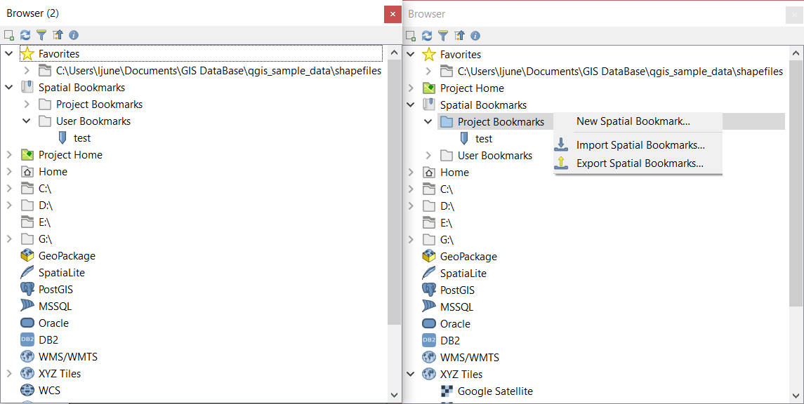
Fig. 11.2 QGIS Browser panels side-by-side
Tip
Add layers to QGIS by simple drag-and-drop from your OS file browser
You can also add file(s) to the project by drag-and-dropping them from your operating system file browser to the Layers Panel or the map canvas.
11.1.2. The DB Manager
The DB Manager Plugin is another tool for integrating and managing spatial database formats supported by QGIS (PostgreSQL, SpatiaLite, GeoPackage, Oracle Spatial, MS SQL Server, Virtual layers). It can be activated from the menu.
The DB Manager Plugin provides several features:
connect to databases and display their structure and contents
preview tables of databases
add layers to the map canvas, either by double-clicking or drag-and-drop.
add layers to a database from the QGIS Browser or from another database
create SQL queries and add their output to the map canvas
create virtual layers
More information on DB Manager capabilities is found in DB Manager Plugin.
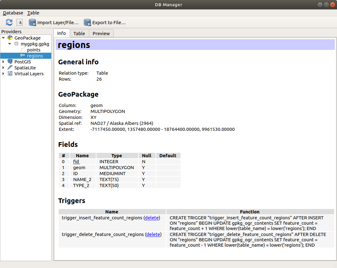
Fig. 11.3 DB Manager dialog
11.1.3. Provider-based loading tools
Beside the Browser Panel and the DB Manager, the main tools provided by QGIS to add layers, you’ll also find tools that are specific to data providers.
Note
Some external plugins also provide tools to open specific format files in QGIS.
11.1.3.1. Loading a layer from a file
To load a layer from a file:
Open the layer type tab in the Data Source Manager dialog, ie click the
Open Data Source Manager
button (or press Ctrl+L) and enable the target tab or:for vector data (like GML, ESRI Shapefile, Mapinfo and DXF layers): press Ctrl+Shift+V, select the
 Add Vector Layer menu option or
click on the Add Vector Layer toolbar button.
Add Vector Layer menu option or
click on the Add Vector Layer toolbar button.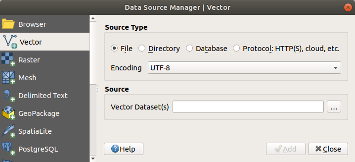
Fig. 11.4 Add Vector Layer Dialog
for raster data (like GeoTiff, MBTiles, GRIdded Binary and DWG layers): press Ctrl+Shift+R, select the
 Add Raster Layer menu option or
click on the Add Raster Layer toolbar button.
Add Raster Layer menu option or
click on the Add Raster Layer toolbar button.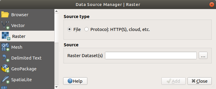
Fig. 11.5 Add Raster Layer Dialog
Check
 File source type
Click on the … Browse button
Navigate the file system and load a supported data source. More than one layer can be loaded at the same time by holding down the Ctrl key and clicking on multiple items in the dialog or holding down the Shift key to select a range of items by clicking on the first and last items in the range. Only formats that have been well tested appear in the formats filter. Other formats can be loaded by selecting
All files(the top item in the pull-down menu).Press Open to load the selected file into Data Source Manager dialog.
Depending on the selected layer type, additional Options (encoding, geometry type, table filtering, file locking, data formatting …) are available for configuring. These options are described in detail in the specific GDAL vector or raster driver documentation. At the top of the options, a text with hyperlink will directly lead to the documentation of the appropriate driver for the selected file format.
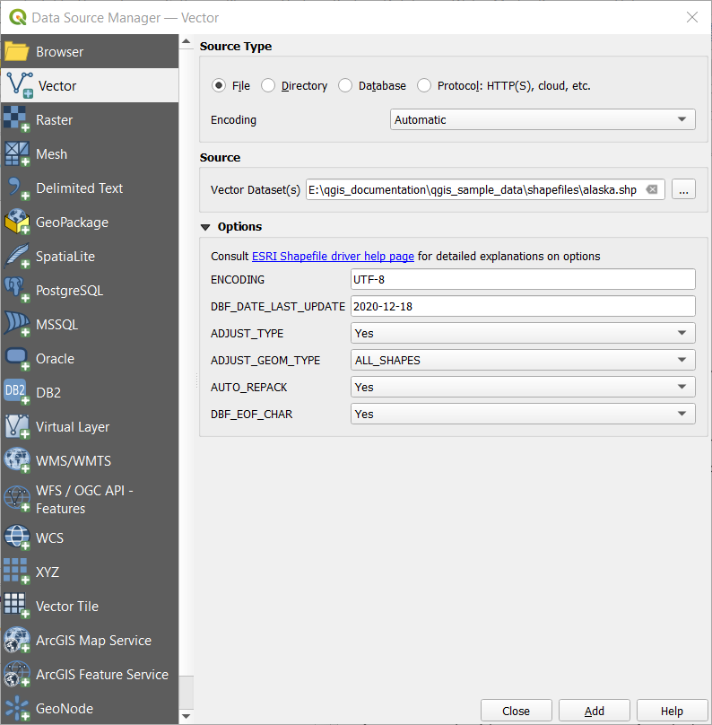
Fig. 11.6 Loading a Shapefile with open options
Press Add to load the file in QGIS and display them in the map view. When adding vector datasets containing multiple layers, the Select Items to Add dialog will appear. In this dialog, you can choose the specific layers from your dataset that you want to add. Also, under Options you can choose to:
 Add layers to a group
- Show system and internal tables
- Show empty vector layers.
Fig. 11.7 shows QGIS after loading the
alaska.shpfile.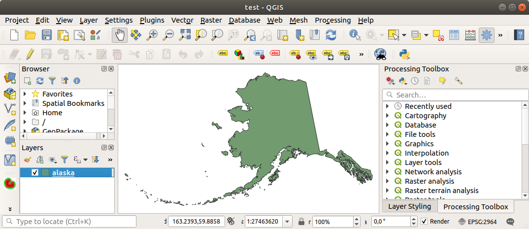
Fig. 11.7 QGIS with Shapefile of Alaska loaded
Note
Because some formats like MapInfo (e.g., .tab) or Autocad (.dxf)
allow mixing different types of geometry in a single file, loading such
datasets opens a dialog to select geometries to use in order to have one
geometry per layer.
The Add Vector Layer and Add Raster
Layer tabs allow loading of layers from source types other than File:
You can load specific vector formats like
ArcInfo Binary Coverage,UK. National Transfer Format, as well as the raw TIGER format of theUS Census BureauorOpenfileGDB. To do that, you select Directory as Source type.
In this case, a directory can be selected in the dialog after pressing
… Browse.With the
Database source type you can select an
existing database connection or create one to the selected database type.
Some possible database types are ODBC,Esri Personal Geodatabase,MS SQL Serveras well asPostgreSQLorMySQL.Pressing the New button opens the Create a New OGR Database Connection dialog whose parameters are among the ones you can find in Creating a stored Connection. Pressing Open lets you select from the available tables.
The
Protocol: HTTP(S), cloud, etc. source type
opens data stored locally or on the network, either publicly accessible,
or in private buckets of commercial cloud storage services.
Supported protocol types are:HTTP/HTTPS/FTP, with a URI and, if required, an authentication.Cloud storage such as
AWS S3,Google Cloud Storage,Microsoft Azure Blob,Microsoft Azure Data Lake Storage,Alibaba OSS Cloud, andOpen Stack Swift Storagesupports direct control over VSI Credential Options when adding OGR vector or GDAL raster layers. You need to fill in the Bucket or container and the Object key first. After that, you can add the necessary Credential Options.When adding OGR vector or GDAL raster layers from the cloud based protocols, you can also set additional Credential options for that specific driver and bucket. When credential options are found in a layer’s URI, they will also be automatically set. This allows different layers to use different credentials.
service supporting OGC
WFS 3(still experimental), usingGeoJSONorGEOJSON - Newline Delimitedformat or based onCouchDBdatabase. A URI is required, with optional authentication.For all vector source types it is possible to define the Encoding or to use the setting.
The
OGC API source type allows you to access
vector
and raster data
from servers that implement the OGC API standards.
To use this option:Select
OGC API from the Data Source Manager
dialog.Enter the endpoint of the OGC API service you want to connect to. Note that you don’t need to prefix the endpoint with “OGCAPI:”.
Click Connect to establish a connection to the server.
11.1.3.2. Loading a mesh layer
A mesh is an unstructured grid usually with temporal and other components. The spatial component contains a collection of vertices, edges and faces in 2D or 3D space. More information on mesh layers at Working with Mesh Data.
To add a mesh layer to QGIS:
Open the dialog, either by selecting it from the menu or clicking the
Open Data Source Manager button.Enable the
 Mesh tab on the left panel
Press the … Browse button to select the file. Various formats are supported.
Select the file and press Add. The layer will be added using the native mesh rendering.
If the selected file contains many mesh layers, then you’ll be prompted with a dialog to choose the sublayers to load. Do your selection and press OK and the layers are loaded with the native mesh rendering. It’s also possible to load them within a group.
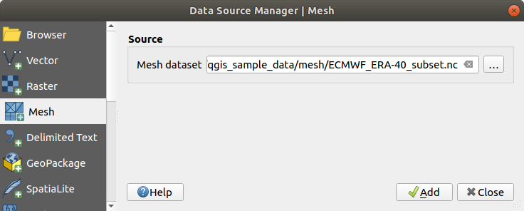
Fig. 11.8 Mesh tab in Data Source Manager
11.1.3.3. Importing a delimited text file
Delimited text files (e.g. .txt, .csv, .dat,
.wkt) can be loaded using the tools described above.
This way, they will show up as simple tables.
Sometimes, delimited text files can contain coordinates / geometries
that you could want to visualize.
This is what  Add Delimited Text Layer
is designed for.
Add Delimited Text Layer
is designed for.
Click the
Open Data Source Manager icon to
open the Data Source Manager dialogEnable the
Delimited Text tabSelect the delimited text file to import (e.g.,
qgis_sample_data/csv/elevp.csv) by clicking on the … Browse button.Configure the settings to meet your dataset and needs, as explained below.
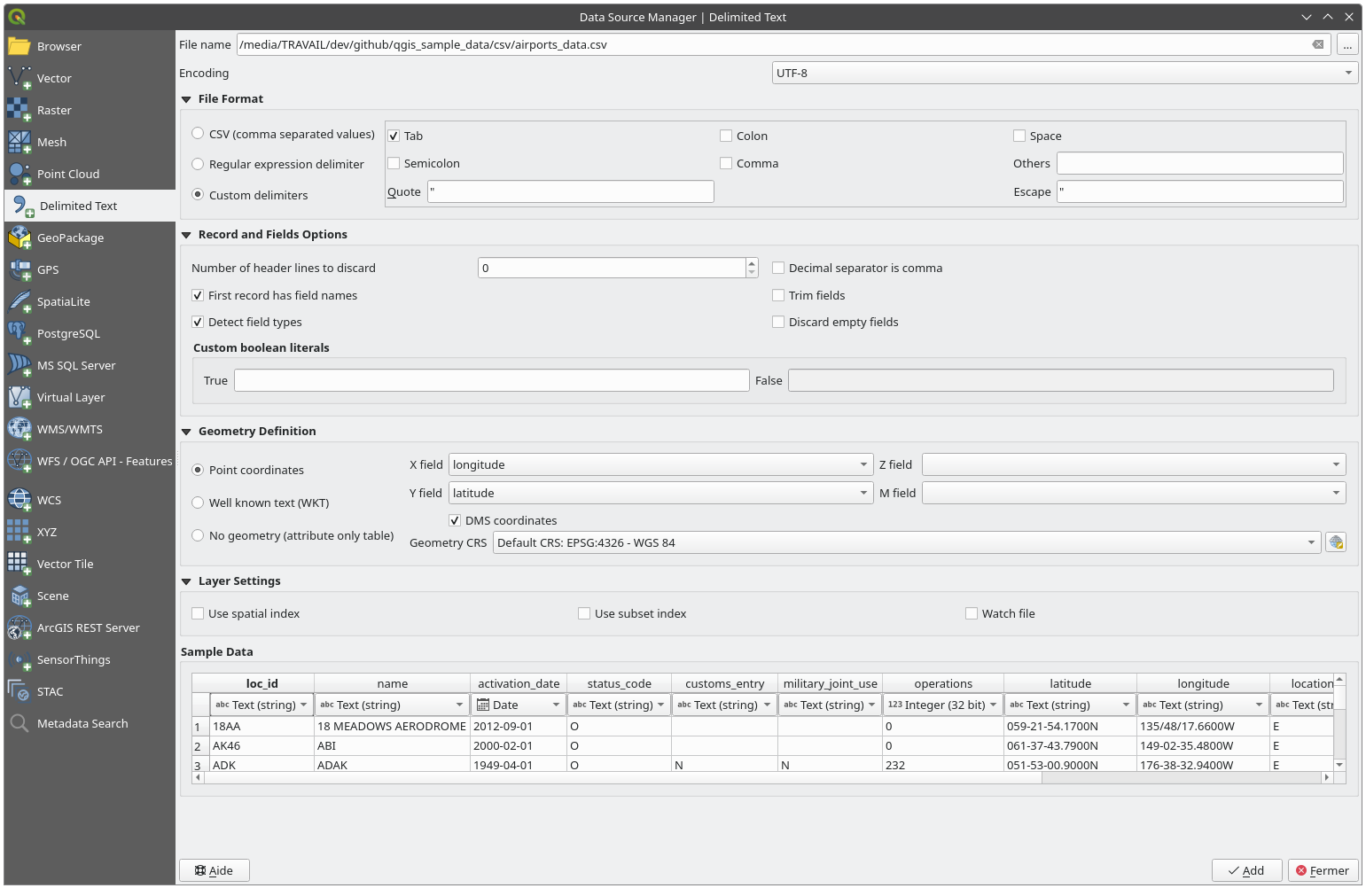
Fig. 11.9 Delimited Text Dialog
File format
Once the file is selected, QGIS attempts to parse the file with the most recently used delimiter, identifying fields and rows. To enable QGIS to correctly parse the file, it is important to select the right delimiter. You can specify a delimiter by choosing between:
- CSV (comma separated values) to use the
comma character.
 Regular expression delimiter and enter text
into the Expression field.
For example, to change the delimiter to tab, use
Regular expression delimiter and enter text
into the Expression field.
For example, to change the delimiter to tab, use \t(this is used in regular expressions for the tab character).- Custom delimiters, choosing among some predefined
delimiters like
comma,space,tab,semicolon, … .
Records and fields
Some other convenient options can be used for data recognition:
Number of header lines to discard: convenient when you want to avoid the first lines in the file in the import, either because those are blank lines or with another formatting.
- First record has field names: values in the first
line are used as field names, otherwise QGIS uses the field names
field_1,field_2… - Detect field types: automatically recognizes the field
type. If unchecked then all attributes are treated as text fields.
- Decimal separator is comma: you can force
decimal separator to be a comma.
- Trim fields: allows you to trim leading and trailing
spaces from fields.
- Discard empty fields.
Custom boolean literals: allows you to add a custom couple of string that will be detected as boolean values.
Field type detection
QGIS tries to detect the field types automatically (unless
Detect field types is not checked) by examining
the content of an optional sidecar CSVT file (see GeoCSV specification)
and by scanning the whole file to make sure that all values can actually
be converted without errors, the fall-back field type is text.
The detected field type appears under the field name in sample data preview table and can be manually changed if necessary.
The following field types are supported:
Booleancase-insensitive literal couples that are interpreted as boolean values are1/0,true/false,t/f,yes/noWhole Number (integer)Whole Number (integer - 64 bit)Decimal Number: double precision floating point numberDateTimeDate and TimeText
Geometry definition
Once the file is parsed, set Geometry definition to
- Point coordinates and provide the X
field, Y field, Z field (for 3-dimensional data)
and M field (for the measurement dimension) if the layer is of
point geometry type and contains such fields. If the coordinates
are defined as degrees/minutes/seconds, activate the
DMS coordinates checkbox.
Provide the appropriate Geometry CRS using the
 Select CRS widget.
 - Well known text (WKT) option if the spatial
information is represented as WKT: select the Geometry field
containing the WKT geometry and choose the appropriate Geometry
field or let QGIS auto-detect it.
Provide the appropriate Geometry CRS using the
Select CRS widget.
If the file contains non-spatial data, activate
No
geometry (attribute only table) and it will be loaded as an ordinary table.
Layer settings
Additionally, you can enable:
- Use spatial index to improve the performance of
displaying and spatially selecting features.
- Use subset index to improve performance of subset
filters (when defined in the layer properties).
- Watch file to watch for changes to the file by other
applications while QGIS is running.
At the end, click Add to add the layer to the map.
In our example, a point layer named Elevation is added to the project
and behaves like any other map layer in QGIS.
This layer is the result of a query on the .csv source file
(hence, linked to it) and would require
to be saved in order to get a spatial layer on disk.
Sample Data
As you set the parser properties, the sample data preview updates regarding to the applied settings.
Also in the Sample Data Table it is possible to override the automatically determined column types.
11.1.3.4. Importing a DXF or DWG file
DXF and DWG files can be added to QGIS by simple drag-and-drop
from the Browser Panel.
You will be prompted to select the sublayers you would like to add
to the project. Layers are added with random style properties.
Note
For DXF files containing several geometry types (point, line and/or polygon), the name of the layers will be generated as <filename.dxf> entities <geometry type>.
To keep the dxf/dwg file structure and its symbology in QGIS, you may want to use the dedicated tool which allows you to:
import elements from the drawing file into a GeoPackage database.
add imported elements to the project.
In the DWG/DXF Import dialog, to import the drawing file contents:
Input the location of the Source drawing, i.e. the DWG/DXF drawing file to import.
Specify the coordinate reference system of the data in the drawing file.
Input the location of the Target package, i.e. the GeoPackage file that will store the data. If an existing file is provided, then it will be overwritten.
Choose how to import
blockswith the dedicated combobox:Expand Block Geometries: imports the blocks in the drawing file as normal elements.
Expand Block Geometries and Add Insert Points: imports the blocks in the drawing file as normal elements and adds the insertion point as a point layer.
Add Only Insert Points: adds the blocks insertion point as a point layer.
Check
Use curves to promote the imported layers
to a curvedgeometry type.Use the Import button to import the drawing into the destination GeoPackage file. The GeoPackage database will be automatically populated with the drawing file content. Depending on the size of the file, this can take some time.
After the .dwg or .dxf data has been imported into the
GeoPackage database, the frame in the lower half of the dialog is
populated with the list of layers from the imported file.
There you can select which layers to add to the QGIS project:
At the top, set a Group name to group the drawing files in the project. By default this is set to the filename of the source drawing file.
Check layers to show: Each selected layer is added to an ad hoc group which contains vector layers for the point, line, label and area features of the drawing layer. The style of the layers will resemble the look they originally had in *CAD.
Choose if the layer should be visible at opening.
Checking the
Merge layers option places all
layers in a single group.Press OK to open the layers in QGIS.
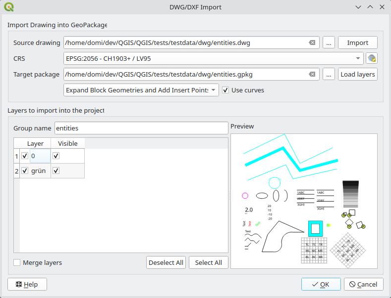
Fig. 11.10 Import dialog for DWG/DXF files
11.1.3.5. Importing OpenStreetMap Vectors
The OpenStreetMap project is popular because in many countries no free geodata such as digital road maps are available. The objective of the OSM project is to create a free editable map of the world from GPS data, aerial photography and local knowledge. To support this objective, QGIS provides support for OSM data.
Using the Browser Panel, you can load an .osm file to the
map canvas, in which case you’ll get a dialog to select sublayers based on the
geometry type.
The loaded layers will contain all the data of that geometry type
in the .osm file, and keep the osm file data structure.
11.1.3.6. SpatiaLite Layers
 The first time you load data from a SpatiaLite
database, begin by:
The first time you load data from a SpatiaLite
database, begin by:
clicking on the
Add SpatiaLite Layer toolbar
buttonselecting the
option from the menuor by typing Ctrl+Shift+L
This will bring up a window that will allow you either to connect to a
SpatiaLite database already known to QGIS (which you choose from the
drop-down menu) or to define a new connection to a new database. To define a
new connection, click on New and use the file browser to point to
your SpatiaLite database, which is a file with a .sqlite extension.
QGIS also supports editable views in SpatiaLite.
11.1.3.7. GPS
There are dozens of different file formats for storing GPS data. The format that QGIS uses is called GPX (GPS eXchange format), which is a standard interchange format that can contain any number of waypoints, routes and tracks in the same file.
Use the … Browse button to select the GPX file, then use the check boxes to select the feature types you want to load from that GPX file. Each feature type will be loaded in a separate layer.
More on GPS data manipulation at Working with GPS Data.
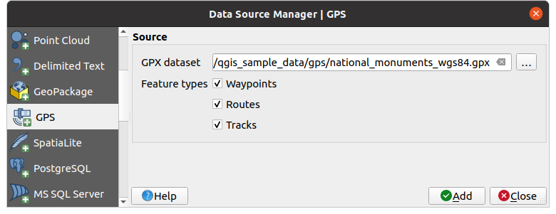
Fig. 11.11 Loading GPS Data dialog
11.1.3.8. GRASS
Working with GRASS vector data is described in section GRASS GIS Integration.
11.1.3.9. Database related tools
Creating a stored Connection
In order to read and write tables from a database format QGIS supports you have to create a connection to that database. While QGIS Browser Panel is the simplest and recommended way to connect to and use databases, QGIS provides other tools to connect to each of them and load their tables:
 or by typing
Ctrl+Shift+D
or by typing
Ctrl+Shift+D or by typing
Ctrl+Shift+O
or by typing
Ctrl+Shift+O
 or by typing
Ctrl+Shift+G
or by typing
Ctrl+Shift+G
These tools are accessible either from the Manage Layers Toolbar and the menu. Connecting to SpatiaLite database is described at SpatiaLite Layers.
Tip
Create connection to database from the QGIS Browser Panel
Selecting the corresponding database format in the Browser tree, right-clicking and choosing connect will provide you with the database connection dialog.
Most of the connection dialogs follow a common structure:
a section with credentials information to connect to the database
a section with options to tune which data can be requested in the database
Connecting to PostgreSQL
The first time you use a PostgreSQL data source, you must create a connection to a database that contains the data. Press the appropriate button as exposed above, opening the PostgreSQL tab of the Data Source Manager dialog. To access the connection manager, click on the New button to display the Create a New PostgreSQL Connection dialog.
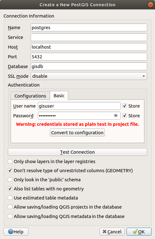
Fig. 11.12 Create a New PostgreSQL Connection Dialog
Name: A name for this connection. It can be the same as Database.
Service: Service parameter to be used alternatively to hostname/port (and potentially database). This can be defined in
pg_service.conf. Check the PostgreSQL Service connection file section for more details.Host: Name of the database host. This must be a resolvable host name such as would be used to open a TCP/IP connection or ping the host. If the database is on the same computer as QGIS, simply enter localhost here.
Port: Port number the PostgreSQL database server listens on. The default port for PostgreSQL is
5432.Database: Name of the database.
SSL mode: SSL encryption setup. The following options are available:
Prefer (the default): I don’t care about encryption, but I wish to pay the overhead of encryption if the server supports it.
Require: I want my data to be encrypted, and I accept the overhead. I trust that the network will make sure I always connect to the server I want.
Verify CA: I want my data encrypted, and I accept the overhead. I want to be sure that I connect to a server that I trust.
Verify Full: I want my data encrypted, and I accept the overhead. I want to be sure that I connect to a server I trust, and that it’s the one I specify.
Allow: I don’t care about security, but I will pay the overhead of encryption if the server insists on it.
Disable: I don’t care about security, and I don’t want to pay the overhead of encryption.
Session role: used to set the current user identifier of the current session. This is useful to automatically give the ownership of a new object (table, view, function) to the session_role group and thus share ownership and associated rights with all members of the session_role group. Read more about session role.
Authentication: For general details about the authentication dialog behavior, see Authentication.
Optionally, depending on the type of database, you can activate the following checkboxes:
- Only show layers in the layer registries
- Don’t resolve type of unrestricted columns (GEOMETRY)
- Also list tables with no geometry:
indicates that tables without geometry should also be listed by default.
- Use estimated table metadata: When initializing layers,
various queries may be needed to establish the characteristics of the geometries
stored in the database table.
When this option is checked, these queries examine only a sample of the rows
and use the table statistics, rather than the entire table.
This can drastically speed up operations on large datasets,
but may result in incorrect characterization of layers
(e.g. the feature count of filtered layers will not be accurately determined)
and may even cause strange behaviour if columns that are supposed to be unique
actually are not.
- Allow saving/loading QGIS projects in the database
- more details here
- Allow saving/loading QGIS layer metadata in the database
- more details here
- Also list raster overview tables
- Only look in the ‘public’ schema
Schema: Allows to specify a single schema to limit a connection to. When set, only tables from the matching schema will be included in the browser panel and data source select for the connection. This can be used to limit the database work required to populate tables for a connection pointing to a large database store.
Once all parameters and options are set, you can test the connection by clicking the Test Connection button or apply it by clicking the OK button.
PostgreSQL Service connection file
The service connection file allows PostgreSQL connection parameters to be associated with a single service name. That service name can then be specified by a client and the associated settings will be used.
It’s called .pg_service.conf under *nix systems (GNU/Linux, macOS etc.)
and pg_service.conf on Windows.
The service file can look like this:
[water_service]
host=192.168.0.45
port=5433
dbname=gisdb
user=paul
password=paulspass
[wastewater_service]
host=dbserver.com
dbname=water
user=waterpass
Note
There are two services in the above example: water_service
and wastewater_service. You can use these to connect from QGIS,
pgAdmin, etc. by specifying only the name of the service you want to
connect to (without the enclosing brackets).
If you want to use the service with psql, you can do psql service=water_service.
You can find all the PostgreSQL parameters here
Note
If you don’t want to save the passwords in the service file you can use the .pg_pass option.
Note
QGIS Server and service
When using a service file and QGIS Server, you must configure the service on the server side as well. You can follow the QGIS Server documentation.
On *nix operating systems (GNU/Linux, macOS etc.) you can save the
.pg_service.conf file in the user’s home directory and
PostgreSQL clients will automatically be aware of it.
For example, if the logged user is web, .pg_service.conf should
be saved in the /home/web/ directory in order to directly work (without
specifying any other environment variables).
You can specify the location of the service file by creating a
PGSERVICEFILE environment variable (e.g. run the
export PGSERVICEFILE=/home/web/.pg_service.conf
command under your *nix OS to temporarily set the PGSERVICEFILE variable).
You can also make the service file available system-wide (all users) either by
placing the .pg_service.conf file in pg_config --sysconfdir or by
adding the PGSYSCONFDIR environment variable to specify the directory
containing the service file. If service definitions with the same name exist
in the user and the system file, the user file takes precedence.
Warning
There are some caveats under Windows:
The service file should be saved as
pg_service.confand not as.pg_service.conf.The service file should be saved in Unix format in order to work. One way to do it is to open it with Notepad++ and .
You can add environmental variables in various ways; a tested one, known to work reliably, is adding
PGSERVICEFILEwith the path - e.g.C:\Users\John\pg_service.confAfter adding an environment variable you may also need to restart the computer.
Connecting to Oracle Spatial
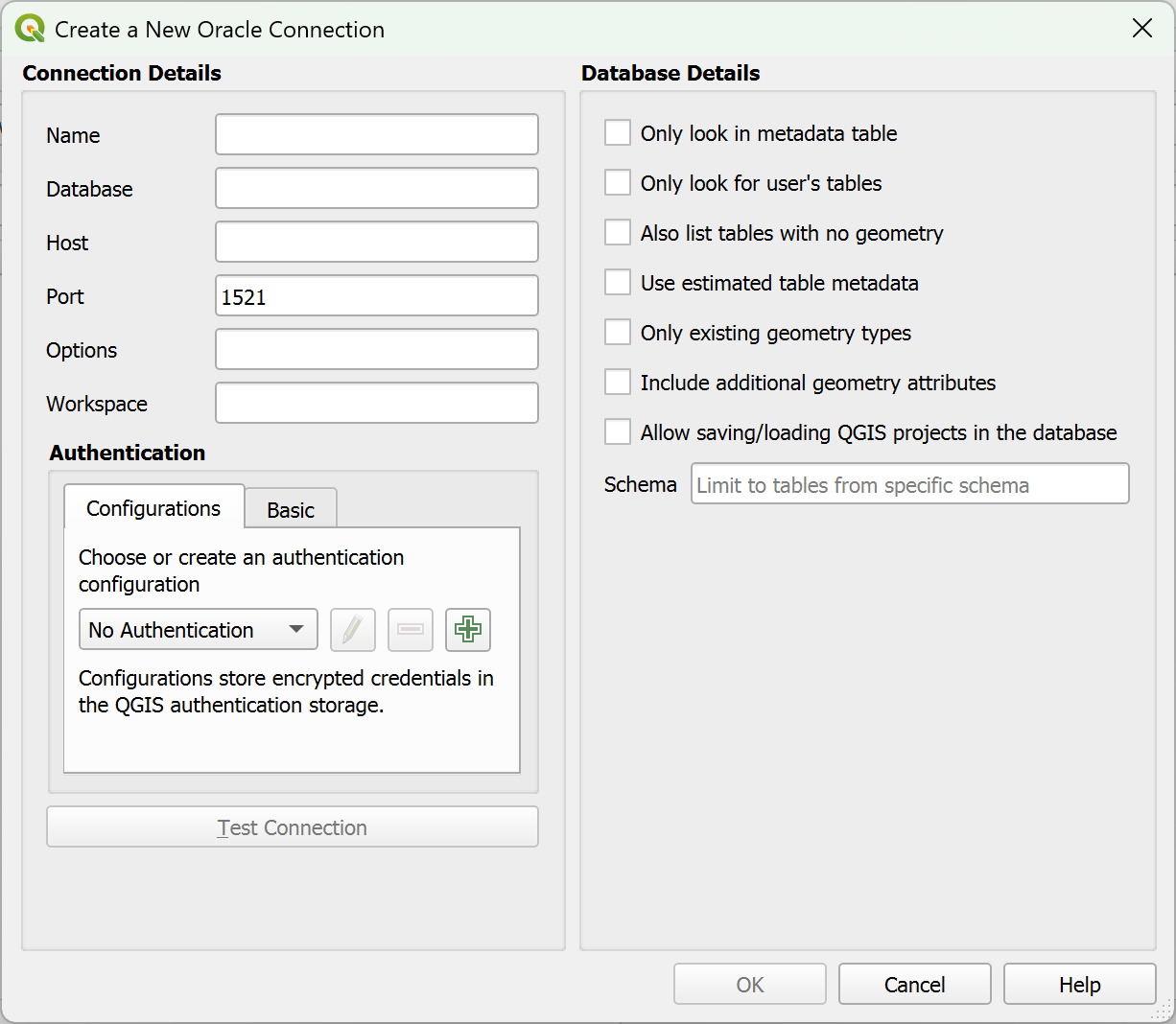
Fig. 11.13 Create a New Oracle Connection Dialog
The spatial features in Oracle Spatial aid users in managing geographic and location data in a native type within an Oracle database. The connection dialog proposes:
Name: A name for this connection. It can be the same as Database;
Database: SID or SERVICE_NAME of the Oracle instance;
Host: The name of the database host;
Port: Port number the Oracle database server listens on. The default port is
1521;Options: Oracle connection specific options (e.g. OCI_ATTR_PREFETCH_ROWS, OCI_ATTR_PREFETCH_MEMORY). The format of the options string is a semicolon separated list of option names or option=value pairs;
Workspace: Workspace to switch to;
Authentication: For general details about the authentication dialog behavior, see Authentication.
Optionally, you can activate the following checkboxes:
- Only look in metadata table: restricts the displayed
tables to those that are in the
all_sdo_geom_metadataview. This can speed up the initial display of spatial tables. - Only look for user’s tables: when searching for spatial tables,
restricts the search to tables that are owned by the user.
- Also list tables with no geometry:
indicates that tables without geometry should also be listed by default.
- Use estimated table statistics for the layer metadata:
when the layer is set up, various metadata are required for the Oracle table.
This includes information such as the table row count, geometry type and
spatial extents of the data in the geometry column.
If the table contains a large number of rows, determining this metadata can be time-consuming.
By activating this option, the following fast table metadata operations are done:
Row count is determined from
all_tables.num_rows. Table extents are always determined with the SDO_TUNE.EXTENTS_OF function, even if a layer filter is applied. Table geometry is determined from the first 100 non-null geometry rows in the table. - Only existing geometry types:
only lists the existing geometry types and don’t offer to add others.
- Include additional geometry attributes.
- Allow saving/loading QGIS projects in the database
- more details here
Schema: Allows to specify a single schema to limit a connection to. When set, only tables from the matching schema will be included in the browser panel and data source select for the connection. This can be used to limit the database work required to populate tables for a connection pointing to a large database store.
Tip
Oracle Spatial Layers
Normally, an Oracle Spatial layer is defined by an entry in the USER_SDO_METADATA table.
To ensure that selection tools work correctly, it is recommended that your tables have a primary key.
Connecting to MS SQL Server
As mentioned in Creating a stored Connection QGIS allows you to create MS SQL Server connection through Data Source Manager.
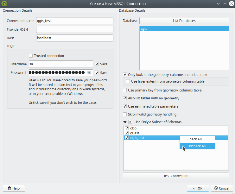
Fig. 11.14 MS SQL Server Connection
To create a new MS SQL Server connection, you need to provide some of the following information in the Connection Details dialog:
Connection name
Provider/DSN
Host
Login information. You can choose to
Save your credentials.
Navigate to the Database Details section and click the List Databases button to view the available datasets. Select datasets that you want, then press OK. Optionally, you can also perform a Test Connection. Once you click OK the Create a New MS SQL Server Connection dialog will close and in the Data Source Manager press Connect, select a layer and then click Add.
Optionally, you can activate the following options:
- Only look in the geometry_columns metadata table:
restricts the available tables to the ones in the
geometry_columnsmetadata table when scanning for tables. This can speed up the table scanning. - Use layer extent from geometry_columns table:
this option, dependent on the previous one, allows QGIS to skip extent calculation
when loading layers and thus lowering the amount of time needed to load them.
It relies on extent manually specified using additional QGIS-specific columns
(
qgis_xmin,qgis_xmax,qgis_ymin,qgis_ymax) in thegeometry_columnstable. - Use primary key from geometry_columns table:
allows QGIS to skip primary key calculation for views when loading them,
thus lowering the amount of time needed to load them.
It relies on names manually filled in a QGIS-specific
qgis_pkeycolumn set in thegeometry_columnstable. If more than one column is used for the primary key, they should be filled as comma separated values. - Also list table with no geometry: tables without a
geometry column attached will also be shown in the available table list.
- Use estimated table parameters: only estimated table
metadata will be used. This avoids a slow table scan, but may result in
incorrect layer properties such as layer extent.
- Skip invalid geometry handling: all handling of records
with invalid geometry will be disabled. This speeds up the provider, however,
if any invalid geometries are present in a table then the result is unpredictable
and may include missing records. Only check this option if you are certain that
all geometries present in the database are valid, and any newly added geometries
or tables will also be valid.
- Use only a Subset of Schemas will allow you to filter
schemas for MS SQL connection. If enabled, only checked schemas will be displayed.
You can right-click to Check or Uncheck any schema in the list.
Renaming a Vector Table (MS SQL)
In Browser Panel, right-click the table and select .
In DB Manager, select the table, then choose .
Connecting to SAP HANA
Note
You require the SAP HANA Client to connect to a SAP HANA database. You can download the SAP HANA Client for your platform at the SAP Development Tools website.
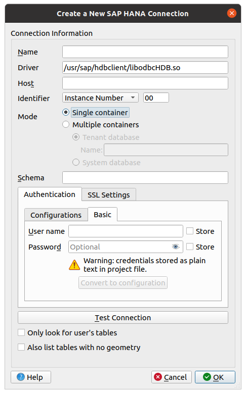
Fig. 11.15 Create a New SAP HANA Connection Dialog
The following parameters can be entered:
Name: A name for this connection.
Driver
 : The name of the HANA ODBC driver. It is
 HDBODBCif you are using 64-bit QGIS,HDBODBC32if you are using 32-bit QGIS. The appropriate driver name is entered automatically.Driver

 : Either the name under which the SAP HANA ODBC
driver has been registered in
: Either the name under which the SAP HANA ODBC
driver has been registered in /etc/odbcinst.inior the full path to the SAP HANA ODBC driver. The SAP HANA Client installer will install the ODBC driver to/usr/sap/hdbclient/libodbcHDB.soby default.Host: The name of the database host.
Identifier: Identifies the instance to connect to on the host. This can be either Instance Number or Port Number. Instance numbers consist of two digits, port numbers are in the range from 1 to 65,535.
Mode: Specifies the mode in which the SAP HANA instance runs. This setting is only taken into account if Identifier is set to Instance Number. If the database hosts multiple containers, you can either connect to a tenant with the name given at Tenant database or you can connect to the system database.
Schema: This parameter is optional. If a schema name is given, QGIS will only search for data in that schema. If this field is left blank, QGIS will search for data in all schemas.
Authentication: For general details about the authentication dialog behavior, see Authentication.
SSL Settings
- Enable TLS/SSL encryption: Enables TLS 1.1 - TLS1.2
encryption. The server will choose the highest available.
Provider: Specifies the cryptographic library provider used for SSL communication. sapcrypto should work on all platforms, openssl should work on
, mscrypto should
work on and commoncrypto requires CommonCryptoLib to be
installed.- Validate SSL certificate: If checked, the SSL
certificate will be validated using the truststore given in
Trust store file with public key.
Override hostname in certificate: Specifies the host name used to verify server’s identity. The host name specified here verifies the identity of the server instead of the host name with which the connection was established. If you specify
*as the host name, then the server’s host name is not validated. Other wildcards are not permitted.Keystore file with private key: Currently ignored. This parameter might allow to authenticate via certificate instead via user and password in future.
Trust store file with public key: Specifies the path to a trust store file that contains the server’s public certificates if using OpenSSL. Typically, the trust store contains the root certificate or the certificate of the certification authority that signed the server’s public certificates. If you are using the cryptographic library CommonCryptoLib or msCrypto, then leave this property empty.
- Only look for user’s tables: If checked, QGIS searches
only for tables and views that are owned by the user that connects to the
database.
- Use estimated table metadata: If checked, estimated
table metadata will be used if available. For large tables, this avoids slow
table loads and potentially expensive computations, but may result in
incorrect layer properties such as layer extent. The fast extent estimation
is available starting with QRC1/2024 and SP8 in HANA Cloud and HANA On-Premise
respectively.
- Also list tables with no geometries: If checked, QGIS
searches also for tables and views that do not contain a spatial column.
Tip
Connecting to SAP HANA Cloud
If you’d like to connect to an SAP HANA Cloud instance, you usually must set
Port Number to 443 and check
Enable TLS/SSL encryption.
Loading a Database Layer
Once you have one or more connections defined to a database (see section Creating a stored Connection), you can load layers from it. Of course, this requires that data are available. See section Importing Data into PostgreSQL for a discussion on importing data into a PostgreSQL database.
To load a layer from a database, you can perform the following steps:
Open the corresponding tab of the database in the Data Source Manager dialog.
Choose the connection name from the drop-down list and press Connect.
The table below will be filled with your data grouped by schema, with a number of metadata information helpful for loading.
Select or unselect
Also list tables with no geometry.Optionally, use some
Search Options to reduce the
list of tables to those matching your search. You can also set this option
before you hit the Connect button, speeding up the database
fetching.Find the layer(s) you wish to add in the list of available layers.
Select it by clicking on it. You can select multiple layers by holding down the Shift or Ctrl key while clicking.
Layers can be selected only if they have no
 warning icon
at the left-hand side of their first column.
This may indicate an issue to detect:
warning icon
at the left-hand side of their first column.
This may indicate an issue to detect:features geometry type: in which case you can select the appropriate one in the drop-down list of the Spatial Type column
layer CRS: you can enter the correct code in the SRID column
layer’s primary key, in order to unequivocally identify each feature: this can be fixed by selecting one or more attributes in the drop-down list at the corresponding Feature id column.
Tip
Use the first column to store “primary keys” for views
Since PostgreSQL views don’t support primary keys, a unique attribute or combination of attributes should always be selected. To help users to speed-up workflows, QGIS automatically selects the first attribute in the view. Therefore, users can define their views in a way that a unique column is in the first position of the view’s definition. In this way, the view will be loaded with no extra interaction and the warning icon will never appear.
If applicable, use the Set Filter button (or double-click the layer) to start the Query Builder dialog (see section Query Builder) and define which features to load from the selected layer. The filter expression appears in the
sqlcolumn. This restriction can be removed or edited in the frame.The checkbox in the
Select at idcolumn that is activated by default gets the feature ids without the attributes and generally speeds up the data loading.Click on the Add button to add the layer to the map.
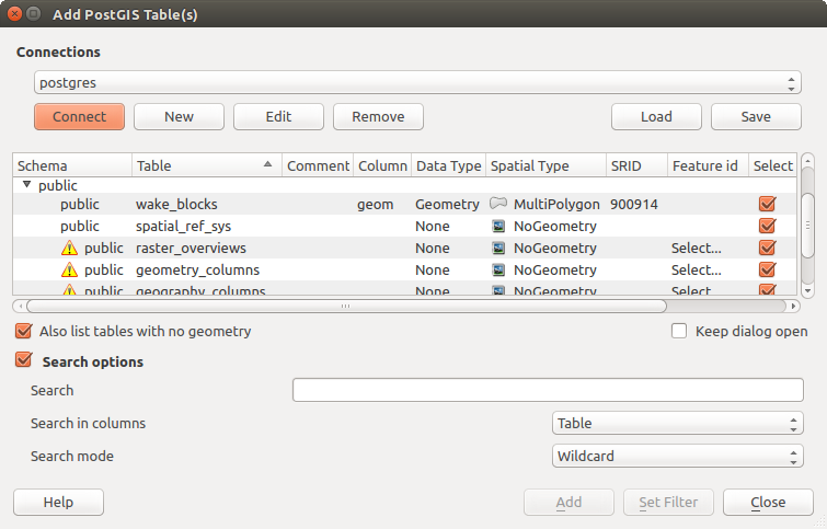
Fig. 11.16 Add PostgreSQL Table(s) Dialog
Tip
Use the Browser Panel to speed up loading of database table(s)
Adding DB tables from the Data Source Manager may sometimes be time consuming as QGIS fetches statistics and properties (e.g. geometry type and field, CRS, number of features) for each table beforehand. To avoid this, once the connection is set, it is better to use the Browser Panel or the DB Manager to drag and drop the database tables into the map canvas.
11.1.4. The Layer Metadata Search Panel
By default, QGIS can retrieve layers metadata from the connections or data providers that allow metadata storage (more details on saving metadata to the database). The Metadata search panel allows to browse the layers by their metadata and add them to the project (either with a double-click or the Add button). The list can be filtered:
by text, watching a set of metadata properties (identifier, title, abstract)
by spatial extent, using the current project extent or the map canvas extent
by the layer (geometry) type
Note
The sources of metadata are implemented through a layer metadata provider system that can be extended by plugins.
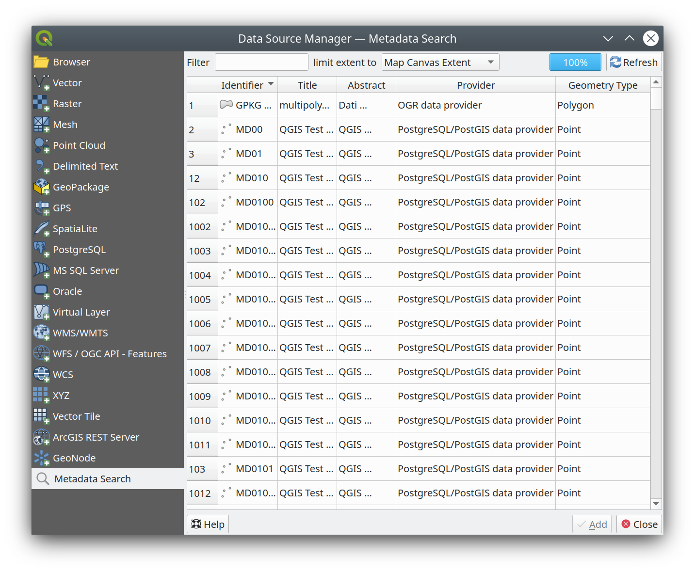
Fig. 11.17 Layer Metadata Search Panel
11.1.5. QGIS Custom formats
QGIS proposes two custom formats:
Temporary Scratch Layer: a memory layer that is bound to the project (see Creating a new Temporary Scratch Layer for more information)
Virtual Layers: a layer resulting from a query on other layer(s) (see Creating virtual layers for more information)
11.1.6. QLR - QGIS Layer Definition File
Layer definitions can be saved as a
Layer Definition File (QLR -
.qlr) using
in the layer
context menu.
The QLR format makes it possible to share “complete” QGIS layers with other QGIS users. QLR files contain links to the data sources and all the QGIS style information necessary to style the layer.
QLR files are shown in the Browser Panel and can be used to add layers (with their saved styles) to the Layers Panel. You can also drag and drop QLR files from the system file manager into the map canvas.
Available actions for QLR files in the Browser Panel are:
Add Layer to Project
Layer Properties…
11.1.7. Connecting to web services
With QGIS you can get access to different types of OGC web services (WM(T)S, WFS(-T), WCS, CSW, …). Thanks to QGIS Server, you can also publish such services. QGIS Server Guide/Manual contains descriptions of these capabilities.
11.1.7.1. Using Vector Tiles services
Vector Tile services can be added via the  Vector
Tiles tab of the Data Source Manager dialog or the contextual menu
of the Vector Tiles entry in the Browser panel.
Services can be either a New Generic Connection… or a
New ArcGIS Vector Tile Service Connection….
Vector
Tiles tab of the Data Source Manager dialog or the contextual menu
of the Vector Tiles entry in the Browser panel.
Services can be either a New Generic Connection… or a
New ArcGIS Vector Tile Service Connection….
You set up a service by adding:
a Name
a Style URL: a URL to a MapBox GL JSON style configuration. If provided, then that style will be applied whenever the layers from the connection are added to QGIS. In the case of Arcgis vector tile service connections, the URL overrides the default style configuration specified in the server configuration.
You can load vector tiles directly from a Style URL. The data source is automatically parsed from the style, and URLs with multiple sources are supported. That makes Source URL optional.
the Source URL: of the type
http://example.com/{z}/{x}/{y}.pbffor generic services andhttp://example.com/arcgis/rest/services/Layer/VectorTileServerfor ArcGIS based services. The service must provide tiles in.pbfformat.the
Min. Zoom Level and the Max. Zoom Level.
Vector Tiles have a pyramid structure. By using these options you have the
opportunity to individually generate layers from the tile pyramid.
These layers will then be used to render the Vector Tile in QGIS.For Mercator projection (used by OpenStreetMap Vector Tiles) Zoom Level 0 represents the whole world at a scale of 1:500.000.000. Zoom Level 14 represents the scale 1:35.000.
the authentication configuration if necessary
a Referer
Fig. 11.18 shows the dialog with the Vector Tiles service configuration.
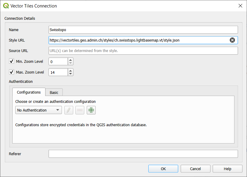
Fig. 11.18 Vector Tiles - Service configuration
Configurations can be saved to .XML file (Save Connections)
through the Vector Tiles entry in Data Source Manager
dialog or its context menu in the Browser panel.
Likewise, they can be added from a file (Load Connections).
Once a connection to a vector tile service is set, it’s possible to:
Edit the vector tile connection settings
Remove the connection
From the Browser panel, right-click over the entry and you can also:
Add layer to project: a double-click also adds the layer
View the Layer Properties… and get access to metadata and a preview of the data provided by the service. More settings are available when the layer has been loaded into the project.
11.1.7.2. Using XYZ Tile services
XYZ Tile services can be added via the  XYZ tab
of the Data Source Manager dialog or the contextual menu of the
XYZ Tiles entry in the Browser panel.
By default, QGIS provides some default and ready-to-use XYZ Tiles services:
XYZ tab
of the Data Source Manager dialog or the contextual menu of the
XYZ Tiles entry in the Browser panel.
By default, QGIS provides some default and ready-to-use XYZ Tiles services:
- Mapzen Global Terrain, allowing an immediate
access to global DEM source for the projects.
More details and resources at https://registry.opendata.aws/terrain-tiles/
- OpenStreetMap to access the world 2D map.
Fig. 11.19 shows the dialog with the OpenStreetMap
XYZ Tile service configuration.
To add a new service, press New (respectively New Connection from the Browser panel) and provide:
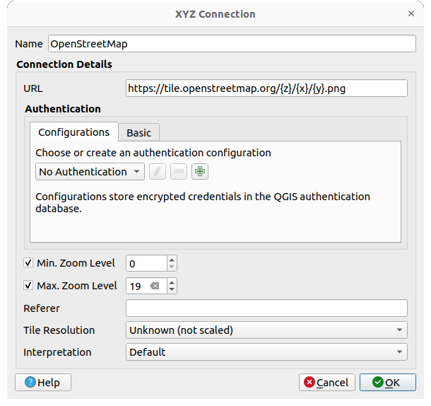
Fig. 11.19 XYZ Tiles - OpenStreetMap configuration
a Name
the URL, you can add
http://example.com/{z}/{x}/{y}.pngorfile:///local_path/{z}/{x}/{y}.pngthe authentication configuration if necessary
the Min. Zoom level and Max. Zoom level
a Referer
the Tile Resolution: possible values are Unknown (not scaled), Standard (256x256 / 96DPI) and High (512x512 / 192DPI)
Interpretation: converts WMTS/XYZ raster datasets to a raster layer of single band float type following a predefined encoding scheme. Supported schemes are Default (no conversion is done), MapTiler Terrain RGB and Terrarium Terrain RGB. The selected converter will translate the RGB source values to float values for each pixel. Once loaded, the layer will be presented as a single band floating point raster layer, ready for styling using QGIS usual raster renderers.
Press OK to establish the connection. It will then be possible to:
Add the new layer to the project; it is loaded with the name given in the settings.
Edit the XYZ connection settings
Remove the connection
From the Browser panel, right-click over the entry and you can also:
Add layer to project: a double-click also adds the layer
View the Layer Properties… and get access to metadata and a preview of the data provided by the service. More settings are available when the layer has been loaded into the project.
Configurations can be saved to .XML file (Save Connections)
through the XYZ entry in Data Source Manager dialog
or its contextual menu in the Browser panel.
Likewise, they can be added from a file (Load Connections).
The XML file for OpenStreetMap looks like this:
<!DOCTYPE connections>
<qgsXYZTilesConnections version="1.0">
<xyztiles url="https://tile.openstreetmap.org/{z}/{x}/{y}.png"
zmin="0" zmax="19" tilePixelRatio="0" password="" name="OpenStreetMap"
username="" authcfg="" referer=""/>
</qgsXYZTilesConnections>
Tip
Loading XYZ tiles without creating a connection
It is also possible to add XYZ tiles to a project without necessarily storing
its connection settings in you user profile (e.g. for a dataset you may need once).
In the tab, edit any properties
in the Connection Details group.
The Name field above should turn into Custom.
Press Add to load the layer in the project.
It will be named by default XYZ Layer.
Examples of XYZ Tile services:
OpenStreetMap Monochrome: URL:
http://tiles.wmflabs.org/bw-mapnik/{z}/{x}/{y}.png, Min. Zoom Level: 0, Max. Zoom Level: 19.Google Maps: URL:
https://mt1.google.com/vt/lyrs=m&x={x}&y={y}&z={z}, Min. Zoom Level: 0, Max. Zoom Level: 19.Open Weather Map Temperature: URL:
http://tile.openweathermap.org/map/temp_new/{z}/{x}/{y}.png?appid={api_key}Min. Zoom Level: 0, Max. Zoom Level: 19.
11.1.7.3. Using ArcGIS REST Servers
An ArcGIS REST Server can host many different types of web services
(feature service, map service, image service, …).
ArcGIS REST Servers can be added via the
 ArcGIS REST Server tab of the
Data Source Manager dialog or the contextual menu of the
ArcGIS REST Servers entry in the Browser panel:
ArcGIS REST Server tab of the
Data Source Manager dialog or the contextual menu of the
ArcGIS REST Servers entry in the Browser panel:
Press New (respectively New Connection) and provide:
a Name: A name for the connection.
the URL: Main address of the ArcGIS REST Server.
a Prefix: Used to specify the proxy prefix in the URL, which is necessary for some ArcGIS servers that use web proxy prefixes.
a Community endpoint URL: Endpoint URL for ArcGIS Online or Portal for ArcGIS, used to access content groups.
a Content endpoint URL: Endpoint URL for the content service. This is used to access items in ArcGIS Online or Portal for ArcGIS.
the authentication credentials if necessary.
a Referer: The referer URL to be sent in the HTTP headers when making requests to the server. This may be required by some servers for authentication purposes.
Note
ArcGIS Feature Service connections which have their corresponding Portal endpoint URLS set can be explored by content groups in the browser panel.
If a connection has the Portal endpoints set, then expanding out the connection in the browser will show a “Groups” and “Services” folder, instead of the full list of services usually shown. Expanding out the groups folder will show a list of all content groups that the user is a member of, each of which can be expanded to show the service items belonging to that group.
Then press OK to validate the configuration settings. These configurations can be saved to
.XMLfile (Save). Likewise, they can be added from a file (Load).Once a connection to an ArcGIS REST Server is set, it is possible to:
Edit the ArcGIS REST Server connection settings
Remove the connection
Refresh the connection
Press Connect to request the server and display its contents. They are organized in a tree structure whose nodes depend on the connection’s endpoint.
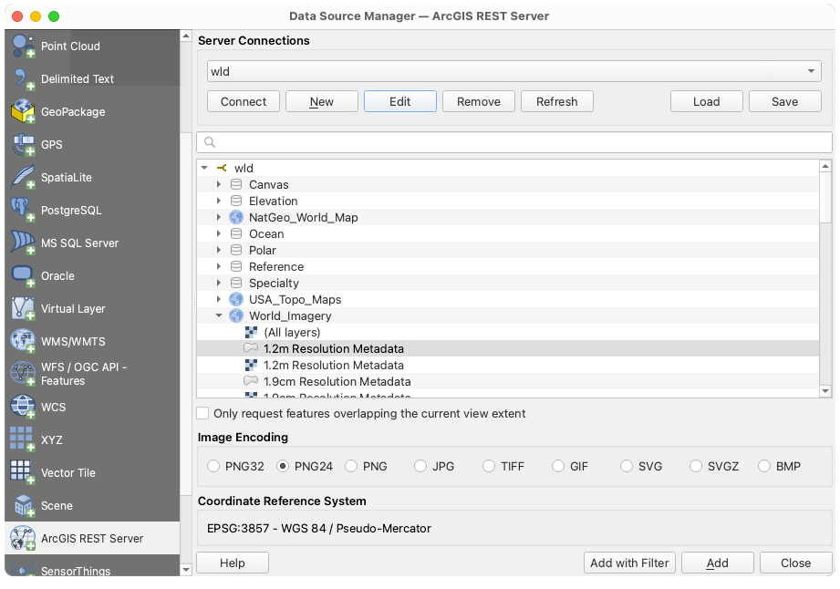
Fig. 11.20 Data Source Manager - ArcGIS REST Server
Expand the tree to find and select the layers of interest. Their Coordinate Reference System is displayed at the bottom of the dialog.
For raster-based layers, you can select the Image encoding to use among a number of image formats advertised by the target service ( e.g.,
PNG,JPG,GIF,SVG,SVGZ, … ).To add the selected layers to the map canvas, press Add button.
Because layers can sometimes load and render slowly on the client side, applying a filter to restrict the features retrieved from the service can significantly improve performance, since only the filtered features are requested from the server. This can be done by:
checking
Only request features overlapping the current view extentfor vector layers (feature service), pressing Add with filter to apply attribute-based filters to the layer with The Expression string builder functions.
In the Browser panel, right-click the ArcGIS REST Server layer and select Add Filtered Layer to Project will also open the builder dialog.
Most of the above tools to connect and access layers on an ArcGIS REST Server are also available from the Browser panel, within the contextual menu of the target node item. Depending on the node, you can also:
View Service Info which will open the default web browser and display information on the requested service.
View the Layer Properties… and get access to the metadata and a preview of the data provided by the service. More settings are available when the layer has been loaded into the project.
11.1.7.4. Using 3D tiled scene services
QGIS supports multiple formats of 3D tiled datasets, grouped together as “tiled scenes”. These include Cesium 3D Tiles and Quantized Mesh tiles.
To load a tiled scene dataset into QGIS, use the  Scene tab in the Data Source Manager dialog.
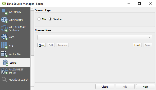
Fig. 11.21 Data Source Manager - Scene
Create a connection by clicking on New. You can add a New Cesium 3D Tiles Connection or a New Quantized Mesh Connection.
Choose a Name and set the URL to the URL of a layer description JSON file.
The URL may be remote (e.g. http://example.com/tileset.json) or local (e.g.
file:///path/to/tiles/tileset.json).
The authentication configuration if necessary.
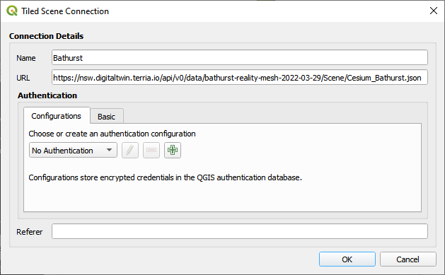
Fig. 11.22 Tiled Scene Connection
You can also add the service from Browser Panel.
After creating new connection you are able to Add the new layer to your map.
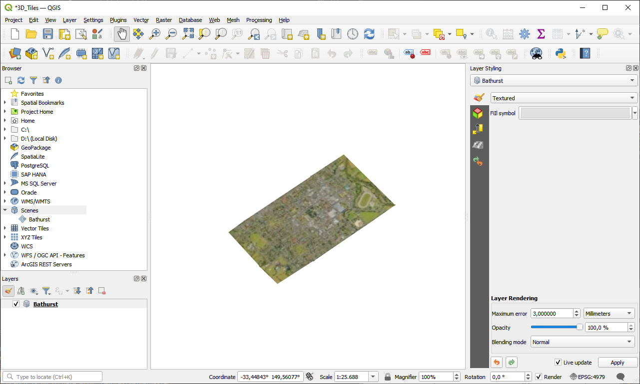
Fig. 11.23 3D Tiles Layer - Textured
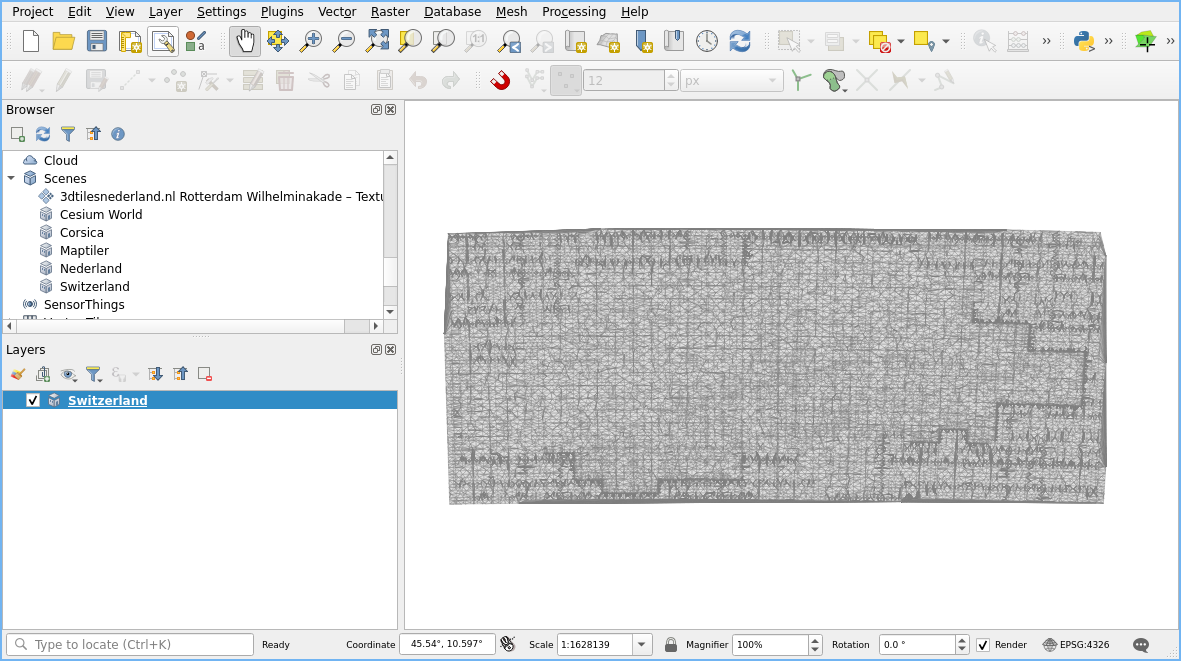
Fig. 11.24 Quantized Mesh layer
11.1.7.5. Using Cloud Connections
QGIS supports connections to cloud services like Alibaba Cloud OSS, Amazon S3, Google Cloud Storage,
Microsoft Azure Blob Storage, Microsoft Azure Data Lake Storage, and OpenStack Swift Object Storage.
You can load vector and raster data from these services into QGIS.
Set up a new  Cloud connection in the Browser panel by right-clicking
on the Cloud entry and selecting New Connection. You will see a drop-down list of
available cloud services.
Select the service you want to connect to and fill in the required fields:
Cloud connection in the Browser panel by right-clicking
on the Cloud entry and selecting New Connection. You will see a drop-down list of
available cloud services.
Select the service you want to connect to and fill in the required fields:
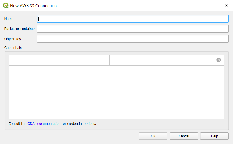
Fig. 11.25 Cloud Connection Dialog
Name: A name for the connection.
Bucket or Container: The name of the bucket or container in the cloud service.
Object Key (optional): The key of the object in the bucket or container.
Credentials: The credentials to access the cloud service.
You can also choose to Save Connection to an XML file or Load Connection from an XML file.
Once a cloud connection is set up, you can right-click on the Cloud entry
in the Browser panel and select Refresh to reload the connection and
update all its sub-elements (e.g. buckets, folders and files).