14.3. Lesson: 수종경계 디지타이즈하기

여러분이 지리참조시킨 맵을 단순히 배경 맵으로 사용할 생각이 아니라면, 다음 단계는 자연스럽게 맵의 요소들을 디지털화하는 일이 됩니다. 여러분은 이미 Lesson: 새 벡터 데이터셋 생성 강의에서 학교 부지를 디지타이즈해서 벡터 데이터를 생성하는 실습을 해봤습니다. 이번 강의에서는, 맵 위에 녹색 라인으로 표출된 수종경계(forest stands)의 경계선을 디지털화하게 될 것입니다. 다만 이번에는 항공사진이 아니라 여러분이 지리참조시킨 맵을 사용할 것입니다.

이 강의의 목표: 디지타이즈 작업, 수종경계 디지타이즈, 그리고 디지타이즈된 수종경계에 목록 데이터 추가하는 데 도움이 되는 기술을 배우기.

14.3.1. Follow Along: 수종경계 경계선 추출

Open your map_digitizing.qgs project in QGIS, that you saved from the previous lesson.

종이 지도를 스캔해서 지리참조시키고 나면 그 이미지를 기준으로 삼아 직접 디지타이즈를 시작할 수 있습니다. 예를 들어 여러분이 디지타이즈할 이미지가 항공사진이라면 거의 그런 방법을 사용하게 되겠죠.

이번 경우처럼 디지타이즈할 이미지가 괜찮은 맵이라면, 각 요소 유형마다 서로 다른 색상이 부여된 라인으로 정보가 명확히 표출되어 있을 것입니다. GIMP 같은 이미지 처리 소프트웨어를 사용하면 이 색상들을 상대적으로 쉽게 개별 이미지로 추출할 수 있습니다. 다음 단계에서 나오겠지만, 이렇게 분리된 이미지는 디지타이즈 작업에 도움이 될 수 있습니다.

첫 번째 단계는 GIMP를 통해 수종경계만 담고 있는 이미지를 얻는 일입니다. 여기서 수종경계란 스캔된 맵 원본에서 볼 수 있는 녹색의 선들을 말합니다.

1. GIMP를 실행하십시오. (아직 설치하지 않았다면 인터넷에서 다운로드하든지 강사에게 문의하십시오.)

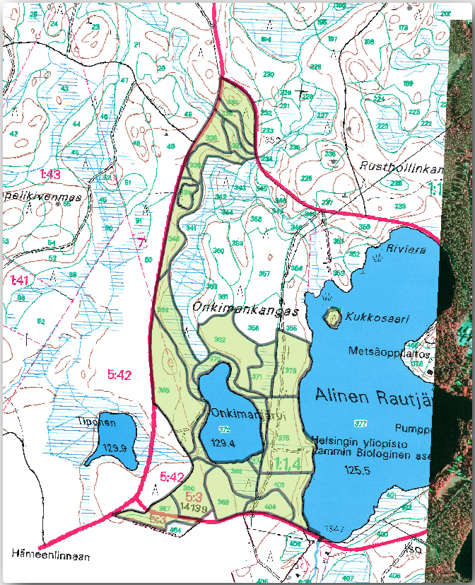
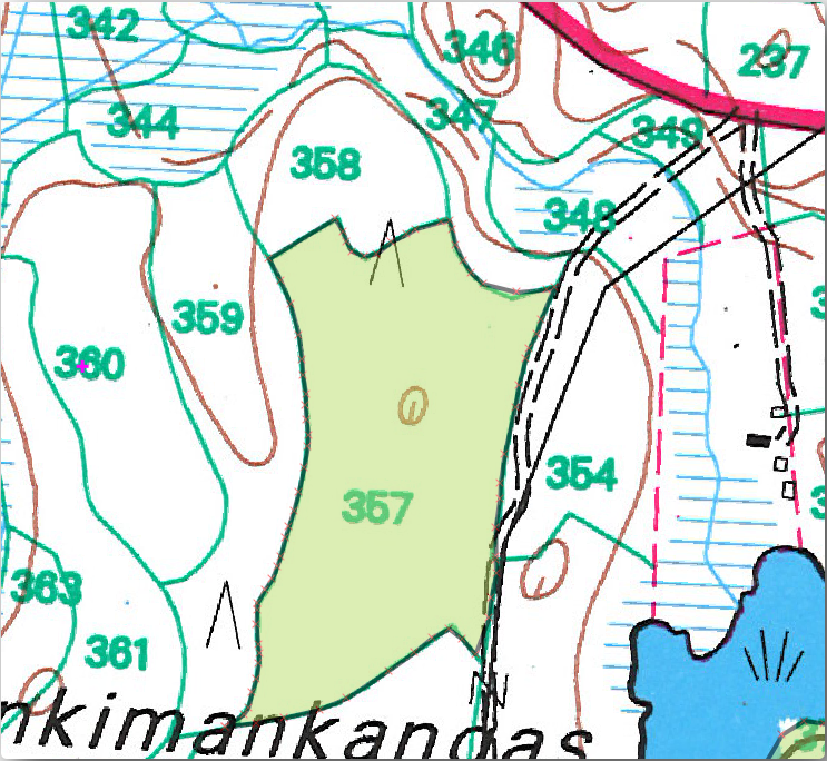
2. Open the original map image, File ► Open, rautjarvi_map.tif in the exercise_data/forestry folder. Note that the forest stands are represented as green lines (with the number of the stand also in green inside each polygon).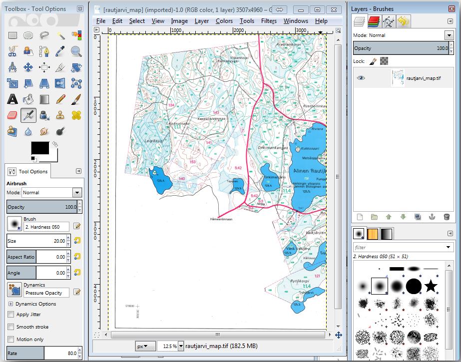

   

   
   

3. 이제 이미지에서 수종경계의 경계선을 표시하는 픽셀(녹색 픽셀)을 선택할 수 있습니다.

   1. 메뉴에서 Select ► By color 도구를 실행하십시오.

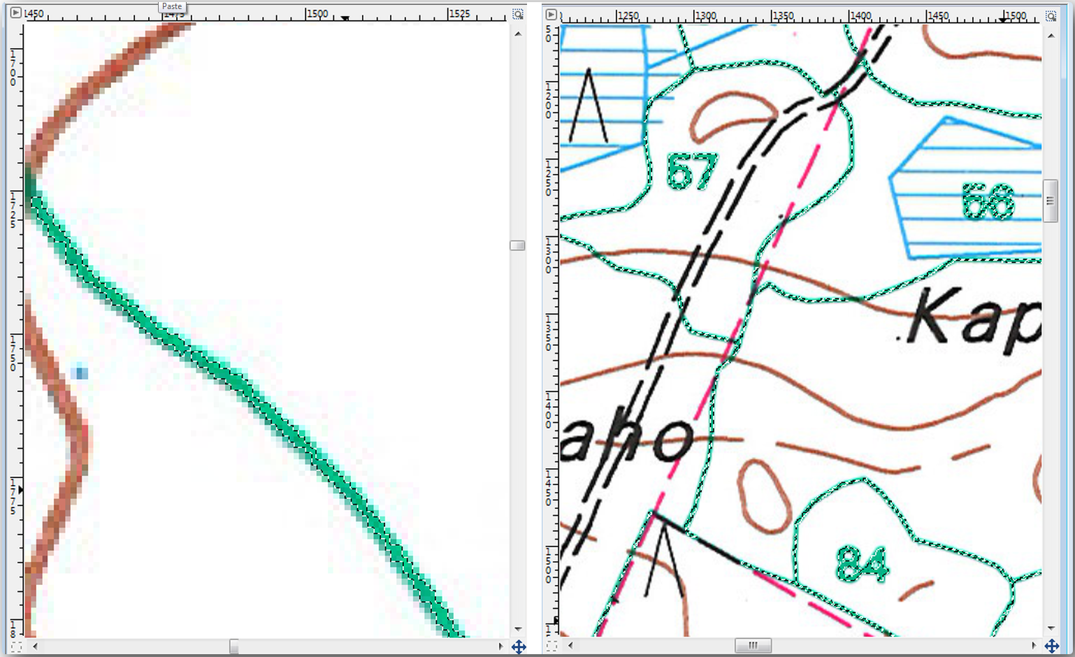
   2. With the tool active, zoom into the image (Ctrl + mouse wheel) so that a forest stand line is close enough to differentiate the pixels forming the line. See the left image below.

   3. 도구가 픽셀의 색상값을 수집할 수 있도록 선 가운데에 마우스 커서를 클릭&드래그하십시오.

   4. 마우스에서 손을 떼고 몇 초 정도 기다리십시오. 도구가 수집한 색상과 일치하는 픽셀들이 이미지 전체에 걸쳐 선택될 것입니다.

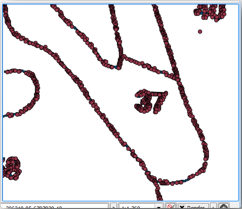
   5. 줌아웃해서 이미지 전체에서 녹색 픽셀들이 어떻게 선택되었는지 살펴보십시오.

   6. 결과물이 마음에 들지 않는다면, 클릭&드래그 작업을 다시 해보십시오.

   7. 여러분이 선택한 픽셀들은 다음 오른쪽 이미지와 비슷하게 보여야 합니다.

   

   
   

4. 선택 작업이 완료됐으면 이 선택한 픽셀들을 새 레이어로 복사해서 개별 이미지 파일로 저장해야 합니다.

   1. Copy (Ctr+C) the selected pixels.

   2. And paste the pixels directly (Ctr+V), GIMP will display the pasted pixels as a new temporary layer in the Layers - Brushes panel as a Floating Selection (Pasted Layer).

   3. 해당 임시 레이어를 오른쪽 클릭한 다음 To New Layer 를 선택하십시오.

   4. 원본 이미지 레이어 옆에 있는 “눈” 아이콘을 클릭해서 레이어를 끄십시오. Pasted Layer 만 보이게 됩니다.

   

   
   

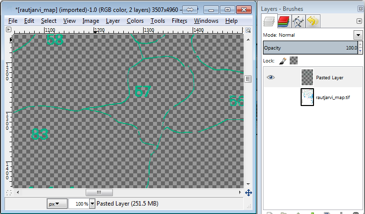
5. Finally, select File ► Export…, set Select File Type (By Extension) as a TIFF image, select the digitizing folder and name it rautjarvi_map_green.tif. Select no compression when asked.

원본 이미지의 다른 요소들도 동일한 과정을 거쳐 추출할 수 있습니다. 예를 들어 도로를 표시하는 검정색 선이나 지형의 등고선을 표시하는 갈색 선을 추출할 수 있습니다. 하지만 이번 강의에서는 수종경계만 사용할 것입니다.

14.3.2. Try Yourself 녹색 픽셀 이미지를 지리참조시키기

이전 강의에서와 마찬가지로, 이 새 이미지를 다른 데이터와 함께 사용하려면 이미지를 지리참조시켜야 합니다.

Note that you don’t need to digitize the ground control points anymore because this image is basically the same image as the original map image, as far as the Georeferencer tool is concerned. Here are some things you should remember:

• This image is also, of course, in KKJ / Finland zone 2 CRS.

• File ► Load GCP points 메뉴를 통해 이전에 저장했던 지상기준점을 사용해야 합니다.

• Transformation settings 를 살펴보는 것을 잊지 마십시오.

• Name the output raster as rautjarvi_green_georef.tif in the digitizing folder.

새 래스터가 원본 맵과 잘 겹치는지 확인하십시오.

14.3.3. Follow Along: 디지타이즈를 위한 보조 포인트 생성

QGIS의 디지타이즈 작업 도구를 떠올려본다면, 디지타이즈 작업을 하는 동안 녹색 픽셀에 스냅하도록 하는 것이 도움이 될 거라고 이미 생각하고 있을 겁니다. 다음 단계는 바로 그렇게 디지타이즈 작업 시 수종경계 경계선을 따라 녹색 픽셀로부터 포인트를 생성하도록 QGIS의 스냅 도구를 이용할 것입니다.

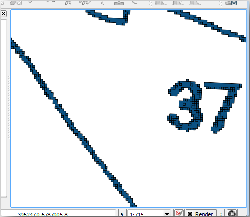
1. Raster ► Conversion ► Polygonize (Raster to Vector) 메뉴를 실행해서 녹색 선을 폴리곤으로 벡터화하십시오. 어떻게 하는지 기억이 안 난다면, Lesson: 래스터 - 벡터 변환 강의를 참조해도 됩니다.

2. Save as rautjarvi_green_polygon.shp inside the digitizing folder.

3. 줌인해서 폴리곤이 어떻게 생겼는지 살펴보십시오. 다음 그림처럼 보일 것입니다.

   

   
   

4. Next option to get points out of those polygons is to get their centroids:

   1. Open Vector ► Geometry Tools ► Centroids….

   2. Set Input Layer to rautjarvi_green_polygon (the polygon layer you have just created)

   3. Set Centroids output to green_centroids.shp file within the folder digitizing

   4. Check Open output file after running algorithm

   5. Press Run. This will calculate the centroids for the polygons as a new layer and add it to the project.

   

   
   

5. Now you can remove the rautjarvi_green_polygon layer from the TOC.

6. Change the symbology of the centroids layer as follows:

   1. Open the Layer Properties for green_centroids.

   2. Symbology 탭을 선택합니다.

   3. Set Size to 1.00 and choose Map Units

각 포인트를 서로 구분지을 필요는 없습니다. 다만 스냅 도구가 포인트를 사용할 수 있기만 하면 됩니다. 이제 이 포인트들을 사용해서 훨씬 쉽게 원본의 선을 딸 수 있을 겁니다.

14.3.4. Follow Along: 수종경계 디지타이즈하기

이제 실제 디지타이즈 작업을 시작할 준비를 마쳤습니다. 먼저 polygon type 의 벡터 파일을 생성해도 되지만, 이 예제에서는 이미 관심 지역의 일부를 디지털화한 shapefile이 존재합니다. 여러분은 주요 도로(굵은 분홍색 선)와 호수 사이에 남아 있는 절반 정도의 수종경계만 디지타이즈하면 됩니다.

1. Go to the digitizing folder using your file manager browser.

2. Drag and drop the forest_stands.shp vector file to your map.

3. Change the new layer’s symbology so that it will be easier to see the polygons that have already been digitized.

   1. Set Fill color to green - and change the Opacity to 50%.

   2. Select Simple Fill and set Stroke width to 1.00 mm.

이전 강의들을 기억한다면, 이제 스냅 옵션을 설정하고 활성화할 차례입니다.

1. Go to Project ► Snapping options…

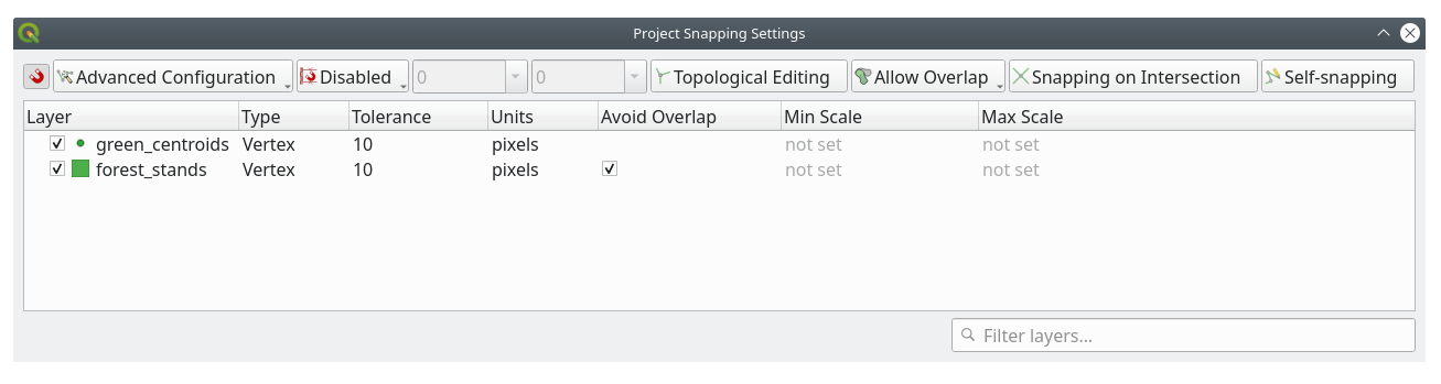
2. Press ^{Enable Snapping} and select Advanced Configuration

3. Check the green_centroids and forest_stands layers

4. Set Type for each layer to Vertex

5. Set Tolerance for each layer to 10

6. Set Units for each layer to pixels

7. Check Avoid Overlap for the forest_stands layer

8. Press Topological editing

9. Choose Follow Advanced Configuration

10. Close the pop-up

    

    With these snapping settings, whenever you are digitizing and get close enough to one of the points in the centroids layer or any vertex of your digitized polygons, a pink square will appear on the point that will be snapped to.

11. Finally, turn off the visibility of all the layers except forest_stands and rautjarvi_georef. Make sure that the map image has not transparency any more.

A few important things to note before you start digitizing:

• 경계선 디지타이즈 작업 시 너무 정확하게 선을 따려 하지 마십시오.

• 경계선이 직선일 경우, 노드 2개만 써서 디지타이즈하십시오. 대개의 경우, 가능한 한 적은 노드를 써서 디지타이즈하십시오.

• 정확하게 작업해야 할 경우에만 근거리로 확대하십시오. 예를 들면 모서리 부분 또는 특정 노드에서 폴리곤과 폴리곤을 접하도록 만들 때 말입니다.

• 디지타이즈 작업 시 마우스 휠을 통해 확대/축소 및 이동을 하십시오.

• 한 번에 폴리곤 하나만 디지타이즈하십시오.

• 하나의 폴리곤 작업이 끝날 때마다 맵 상에 보이는 수종경계 ID를 입력하십시오.

이제 디지타이즈 작업을 시작해봅시다.

1. Locate the forest stand number 357 in the map window.

2. Select the forest_stands layer.

3. Click the ^{Toggle Editing} button to enable editing

4. Select ^{Add Polygon Feature} tool.

5. Start digitizing the stand 357 by connecting some of the dots. Note the pink crosses indicating the snapping.

When you are done:

1. Right click to end digitizing that polygon.

2. Enter the forest stand ID within the form (in this case 357).

3. OK 를 클릭하십시오.

If a form did not appear when you finished digitizing the polygon, go to Settings ► Options ► Digitizing and make sure that the Suppress attribute form pop-up after feature creation is not checked.

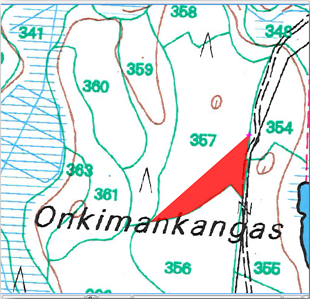
여러분이 디지타이즈한 폴리곤은 다음 그림처럼 보일 것입니다.

Now for the second polygon, pick up the stand number 358. Make sure that Avoid Overlap is checked for the forest_stands layer (as shown above). This option ensures polygons do not overlap. So, if you digitize over an existing polygon, the new polygon will be trimmed to meet the border of the existing polygons. You can use this option to automatically obtain a common border.

1. 수종경계 357과 맞닿은 모서리 가운데 하나로부터 수종경계 358의 디지타이즈 작업을 시작하십시오.

2. Continue normally until you get to the other common corner for both stands.

3. 마지막으로 맞닿는 모서리가 서로 교차하지 않도록 폴리곤 357 내부에 포인트를 몇 개 디지타이즈하십시오. 다음 왼쪽 이미지를 참조하세요.

4. 오른쪽 클릭해서 수종경계 358의 편집을 끝냅니다.

5. Enter the ID as 358.

6. Click OK. Your new polygon should have a common border with the stand 357 as you can see in the image below.

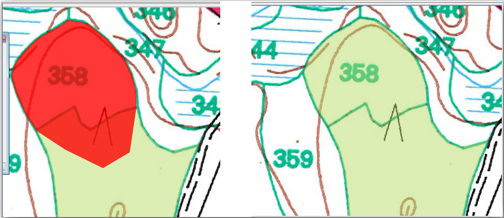
The part of the polygon that was overlapping the existing polygon has been automatically trimmed and you are left with a common border - as you intended it to be.

14.3.5. Try Yourself 수종경계 디지타이즈 끝내기

이제 수종경계 2개를 완료했습니다. 이렇게 해보면 어떨까요? 주요 도로와 호수 사이에 있는 모든 수종경계를 디지털화할 때까지 디지타이즈 작업을 계속하는 겁니다.

힘든 일처럼 보일 수도 있지만, 수종경계를 디지타이즈하는 작업에 금새 익숙해질 겁니다. 15분 정도면 다 끝낼 수 있습니다.

디지타이즈 작업 도중 노드를 편집 또는 삭제하거나, 폴리곤들을 나누거나 합쳐야 할 수도 있습니다. Lesson: 피처의 위상 강의에서 이때 필요한 도구에 대해 배웠습니다. 이제 해당 강의를 다시 읽어보는 게 어떨까요.

Enable topological editing 옵션을 활성화했기 때문에, 두 폴리곤이 맞닿아 있는 노드를 이동시켜 동시에 두 폴리곤의 공통 경계선을 편집할 수도 있다는 사실을 기억하십시오.

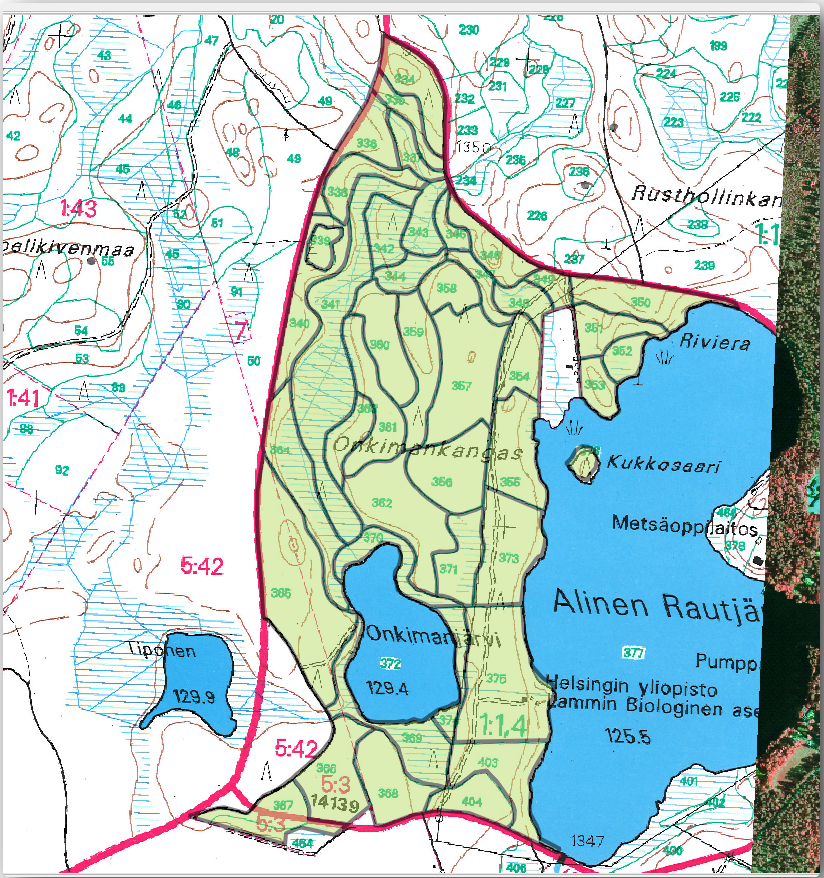
여러분의 산출물이 다음 그림처럼 보여야 합니다.

14.3.6. Follow Along: 수종경계 데이터 합치기

여러분의 맵에 대해 여러분이 가진 삼림 목록 데이터 또한 종이에 기록된 정보일 수도 있습니다. 이럴 경우, 먼저 해당 데이터를 텍스트 파일이나 스프레드시트로 입력해야 합니다. 이번 예제에서는, (맵과 동일한 연도인) 1994년 목록 정보를 쉼표로 구분된 텍스트 파일(csv)로 준비했습니다.

1. Open the rautjarvi_1994.csv file from the exercise_data\forestry directory in a text editor and note that the inventory data file has an attribute called ID that has the numbers of the forest stands. Those numbers are the same as the forest stands ids you have entered for your polygons and can be used to link the data from the text file to your vector file. You can see the metadata for this inventory data in the file rautjarvi_1994_legend.txt in the same folder.

2. Now add this file into the project:

   1. Use the ^{Add Delimited Text Layer} tool. This is accessed via Layer ► Add Layer ► Add Delimited Text Layer….

   2. Set details in the dialog as follows:

      

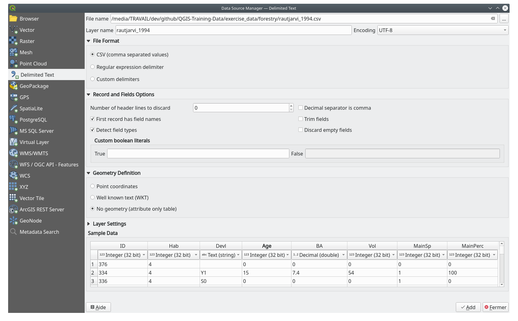
   3. Press Add to load the formatted csv file in the project.

3. To link the data from the .csv file with the digitized polygons, create a join between the two layers:

   1. Open the Layer Properties for the forest_stands layer.

   2. Joins 탭을 선택합니다.

   3. Click ^{Add new join} on the bottom of the dialog box.

   4. Select rautjarvi_1994.csv as the Join layer

   5. Set the Join field to ID

   6. Set the Target field to ID

   7. OK 를 두 번 클릭합니다.

The data from the text file should be now linked to your vector file. To see what has happened, select the forest_stands layer and use ^{Open Attribute Table}. You can see that all the attributes from the inventory data file are now linked to your digitized vector layer.

You will see that the field names are prefixed with rautjarvi_1994_. To change this:

1. Open the Layer Properties for the forest_stands layer.

2. Joins 탭을 선택합니다.

3. Select Join Layer rautjarvi_1994

4. Click the ^{Edit selected join} button to enable editing

5. Under Custom field name prefix remove the prefix name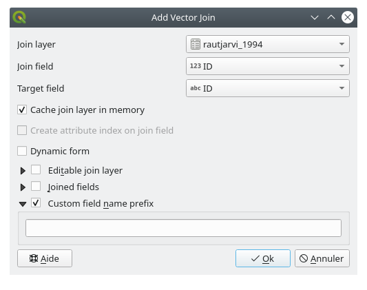

   

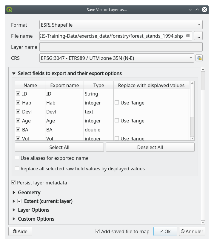
The data from the .csv file is just linked to your vector file. To make this link permanent, so that the data is actually recorded to the vector file you need to save the forest_stands layer as a new vector file. To do this:

1. Right click on forest_stands layer

2. Choose Export ► Save Features As…

3. Set Format to ESRI Shapefile

4. Set file name to forest_stands_1994.shp under the forestry folder

5. To include the new file as a layer in the project, check Add saved file to map

14.3.7. Try Yourself Adding Area and Perimeter

To finish gathering the information related to these forest stands, you might calculate the area and the perimeter of the stands. You calculated areas for polygons in Lesson: 보충 예제. Go back to that lesson if you need to and calculate the areas for the forest stands. Name the new attribute Area and make sure that the values calculated are in hectares. You could also do the same for the perimeter.

Now your forest_stands_1994 layer is ready and packed with all the available information.

Save your project to keep the current map layers in case you need to come back later to it.

14.3.8. In Conclusion

마우스 클릭을 많이 해야 했지만, 이제 옛날 목록 데이터를 디지털 형식으로 바꾸어 QGIS에서 이용할 준비를 끝냈습니다.

14.3.9. What’s Next?

새로 만든 데이터셋으로 다른 분석을 할 수도 있지만, 좀 더 최신 정보로 업데이트된 데이터셋으로 분석을 수행하고 싶을 것입니다. 다음 강의의 주제는 최신 항공사진을 이용해서 수종경계를 생성하고 몇몇 관련 정보를 사용자의 데이터셋에 추가하는 것입니다.