14.3. Lesson: Digitalizando Massas Florestais

A menos que você vá usar seu mapa georreferenciado como uma simples imagem de fundo, o próximo passo natural é digitalizar os elementos dele. Você já fez isso nos exercícios sobre como criar dados vetoriais em ../criar/dados_vetoriais /criar_novo_vetor, quando você digitalizou os campos da escola. Nesta lição, você irá digitalizar as bordas dos povoamentos florestais que aparecem no mapa como linhas verdes, mas em vez de fazer isso usando uma imagem aérea, você usará seu mapa georreferenciado.

El objetivo de esta lección: Aprender una técnica para asistir la tarea de digitalización, digitalizar una masa forestal y finalmente añadirle los datos de inventario.

14.3.1. Follow Along: Extrayendo los Bordes de las Masas Forestales

Open your map_digitizing.qgs project in QGIS, that you saved from the previous lesson.

Una vez escaneado y georeferenciado tu mapa podría empezar a digitalizarse directamente mirando las imágenes a modo de guía. Esa sería la forma más adecuada si la imagen desde la que vas a digitalizar es, por ejemplo, una fotografía aérea.

Se o que você está usando para digitalizar é um bom mapa, como é o nosso caso, é provável que as informações sejam exibidas claramente como linhas com cores diferentes para cada tipo de elemento. Essas cores podem ser extraídas com relativa facilidade como imagens individuais usando um software de processamento de imagem como o GIMP. Essas imagens separadas podem ser usadas para auxiliar na digitalização, como você verá abaixo.

El primer paso será utilizar GIMP para obtener una imagen que contenga solo las masas forestales, es decir, todas las líneas verdosas que podrías ver en el mapa original escaneado:

1. Abre GIMP (si todavía no lo has instalado, descárgatelo de internet o pregunta a tu profesor).

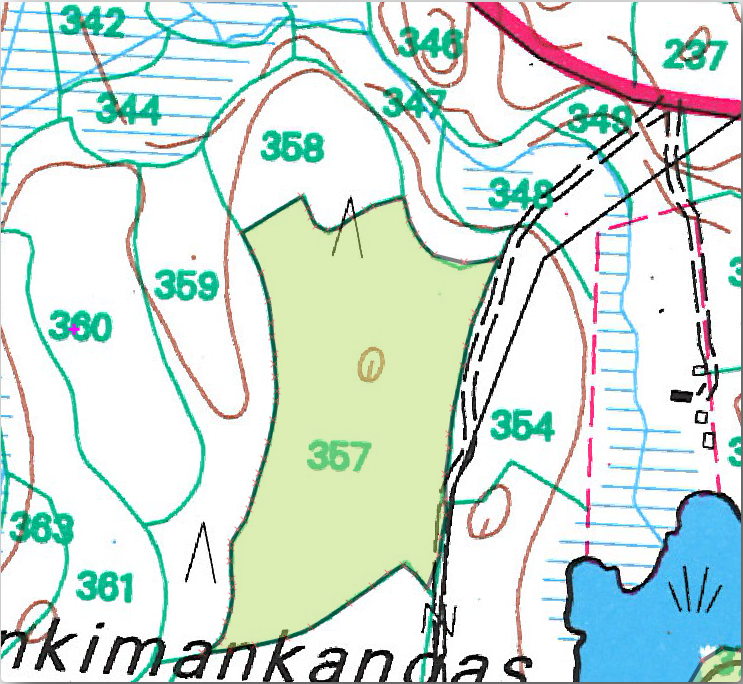
2. Open the original map image, File ► Open, rautjarvi_map.tif in the exercise_data/forestry folder. Note that the forest stands are represented as green lines (with the number of the stand also in green inside each polygon).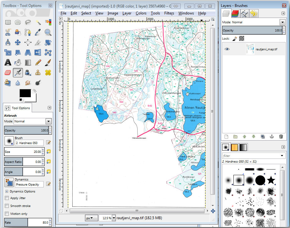

   

   
   

3. Agora você pode selecionar os pixels na imagem que formam os limites das massas florestais (os pixels esverdeados):

   1. Abre la herramienta Select ► By color.

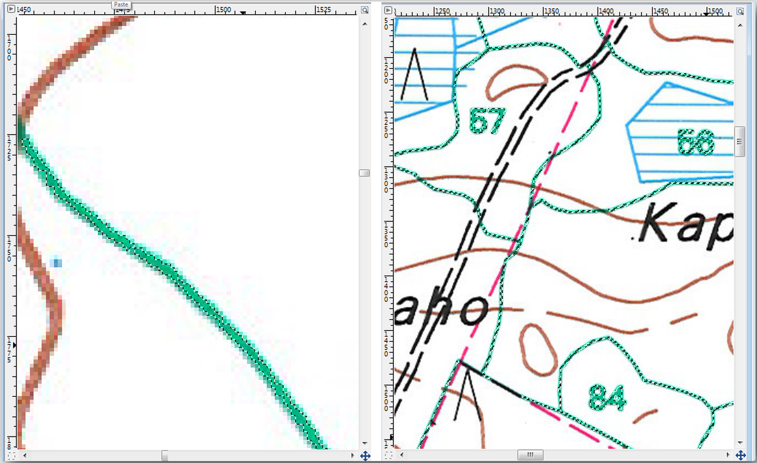
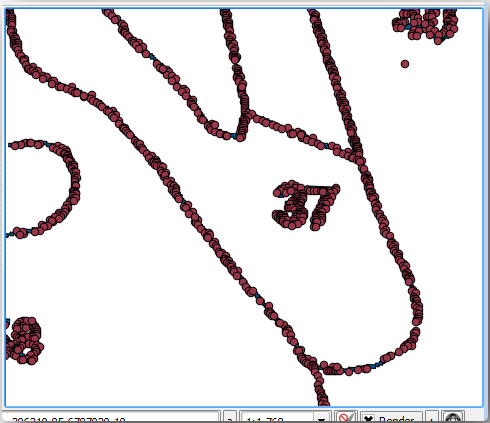
   2. With the tool active, zoom into the image (Ctrl + mouse wheel) so that a forest stand line is close enough to differentiate the pixels forming the line. See the left image below.

   3. Haz clic y arrastra el cursor del ratón en el medio de la línea para que la herramienta recolecte muchos valores de color de píxel.

   4. Deja de clicar y espera unos segundos. Los píxeles que coincidan con los colores recogidos por la herramienta serán seleccionados en toda la imagen.

   5. Aleja el zum para ver como los píxeles verdosos se han seleccionado en toda la imagen.

   6. Si no estas contento con tus resultados, repite la operación de clicado y arrastrar.

   7. Sua seleção de pixels deve ficar parecida com a imagem abaixo à direita.

   

   
   

4. Una vez hayas terminado con la selección necesitas copiar la selección como una capa nueva y guardarla como un archivo de imagen separado:

   1. Copy (Ctr+C) the selected pixels.

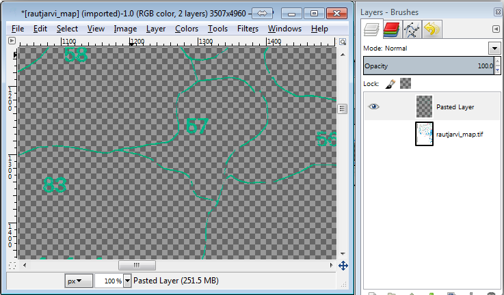
   2. And paste the pixels directly (Ctr+V), GIMP will display the pasted pixels as a new temporary layer in the Layers - Brushes panel as a Floating Selection (Pasted Layer).

   3. Haz clic derecho en la capa temporal y selecciona To New Layer.

   4. Haz clic en el icono “eye” junto a la capa original para desactivarlo, para que solo sea visible la Pasted Layer:

   

   
   

5. Finally, select File ► Export…, set Select File Type (By Extension) as a TIFF image, select the digitizing folder and name it rautjarvi_map_green.tif. Select no compression when asked.

Podrías hacer el mismo proceso con otros elementos de la imagen, por ejemplo para extraer las líneas negras que representan calles o las marrones que representan las líneas de contorno del terreno. Pero para nosotros, con las masas forestales es suficiente.

14.3.2. Try Yourself georeferenciar la Imagen de píxeles Verdes

Como hiciste en la lección anterior, necesitas georeferenciar esta nueva imagen para ser capaz de utilizarla con el resto de tus datos.

Note that you don’t need to digitize the ground control points anymore because this image is basically the same image as the original map image, as far as the Georeferencer tool is concerned. Here are some things you should remember:

• This image is also, of course, in KKJ / Finland zone 2 CRS.

• Deberías utilizar los puntos de control base que guardaste, File ► Load GCP points.

• Lembre-se de rever Transformation settings.

• Name the output raster as rautjarvi_green_georef.tif in the digitizing folder.

Comprueba que el nuevo ráster encaja bien en el mapa original.

14.3.3. Follow Along: Creando Puntos de Soporte para Digitalizar

Tendo em mente as ferramentas de digitalização do QGIS, você já pode ter pensado que seria útil ter o snap para esses pixels verdes enquanto digitaliza. Isso é precisamente o que você vai fazer agora: criar pontos a partir desses pixels para usá-los depois para ajudá-lo a seguir as fronteiras das florestas enquanto digitaliza, usando as ferramentas de snap disponíveis no QGIS.

1. Utiliza la herramienta Raster ► Conversion ► Polygonize (Raster to Vector) para vectorizar tus líneas verdes a polígonos. Si no recuerdas cómo, puedes repasarlo en el módulo 9.1.1.

2. Save as rautjarvi_green_polygon.shp inside the digitizing folder.

3. Amplía el zum y observa como se ven los polígonos. Obtendrás algo como esto:

   

   
   

4. Next option to get points out of those polygons is to get their centroids:

   1. Open Vector ► Geometry Tools ► Centroids….

   2. Set Input Layer to rautjarvi_green_polygon (the polygon layer you have just created)

   3. Set Centroids output to green_centroids.shp file within the folder digitizing

   4. Check Open output file after running algorithm

   5. Press Run. This will calculate the centroids for the polygons as a new layer and add it to the project.

   

   
   

5. Now you can remove the rautjarvi_green_polygon layer from the TOC.

6. Change the symbology of the centroids layer as follows:

   1. Open the Layer Properties for green_centroids.

   2. Vá para a guia Simbologia.

   3. Set Size to 1.00 and choose Map Units

No es necesario diferenciar los puntos entre ellos, solo necesitas que estén ahí para que las herramientas de rotura los utilicen. Puedes utilizar esos puntos ahora para seguir las líneas originales mucho más fácil que sin ellos.

14.3.4. Follow Along: Digitaliza las Masas Forestales

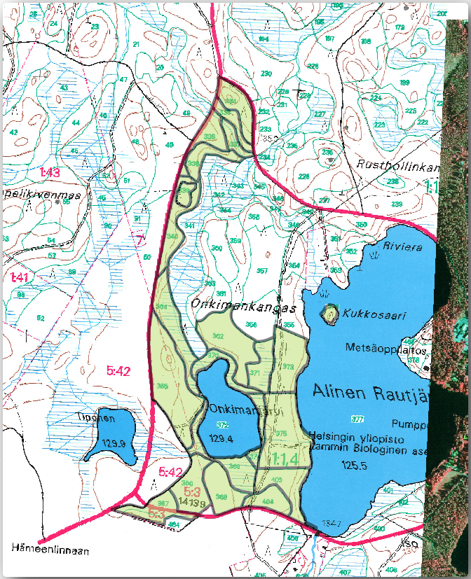
Ahora estás listo para empezar con el trabajo de digitalización. Empezarías creando un archivo vectorial de polygon type, pero para este ejercicio, hay un archivo shape con parte del área de interés ya digitalizada. Terminarás de digitalizar la mitad de las masas forestales que se ha dejado entre las calles principales (líneas anchas rosas) y el lago:

1. Go to the digitizing folder using your file manager browser.

2. Drag and drop the forest_stands.shp vector file to your map.

3. Change the new layer’s symbology so that it will be easier to see the polygons that have already been digitized.

   1. Set Fill color to green - and change the Opacity to 50%.

   2. Select Simple Fill and set Stroke width to 1.00 mm.

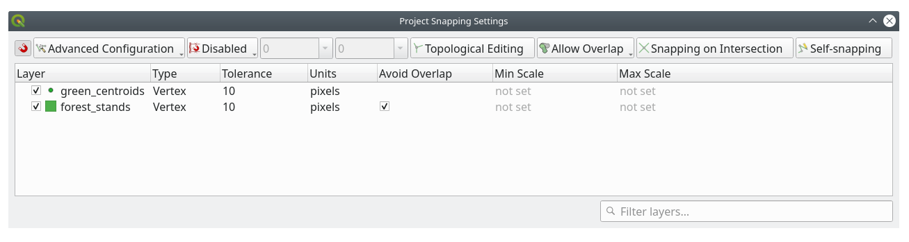
Ahora, si recuerdas los módulos anteriores, tenemos que ajustar y activar las opciones de rotura:

1. Go to Project ► Snapping options…

2. Press ^{Enable Snapping} and select Advanced Configuration

3. Check the green_centroids and forest_stands layers

4. Set Type for each layer to Vertex

5. Set Tolerance for each layer to 10

6. Set Units for each layer to pixels

7. Check Avoid Overlap for the forest_stands layer

8. Press Topological editing

9. Choose Follow Advanced Configuration

10. Close the pop-up

    

    With these snapping settings, whenever you are digitizing and get close enough to one of the points in the centroids layer or any vertex of your digitized polygons, a pink square will appear on the point that will be snapped to.

11. Finally, turn off the visibility of all the layers except forest_stands and rautjarvi_georef. Make sure that the map image has not transparency any more.

A few important things to note before you start digitizing:

• No intentes ser demasiado preciso con la digitalización de los bordes.

• Si un borde es una línea recta, digitalízala con solo dos nodos. En general, digitaliza utilizando el menor número de nodos posible.

• Amplía el zum a rangos cercanos solo si crees que necesitas ser preciso, por ejemplo, en algunas esquitas o cuando quieres que un polígono conecte con otro en un cierto nodo.

• Utiliza el botón medio del ratón para amliar y reducir el zum y desplazarte mientras digitalizas.

• Digitaliza solo un polígono de cada vez

• Después de digitalizar un polígono, escribe la identidad de masa forestal que puedes ver en el mapa.

Ahora puedes empezar a digitalizar:

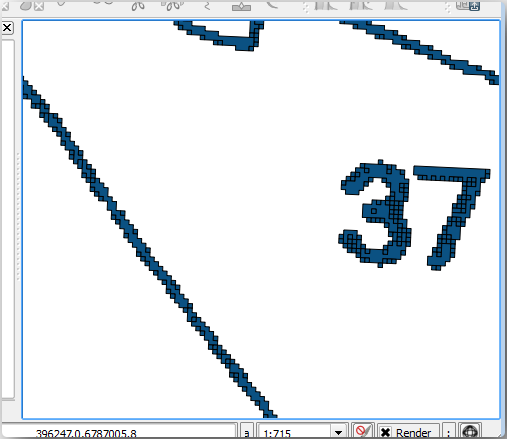
1. Locate the forest stand number 357 in the map window.

2. Select the forest_stands layer.

3. Click the ^{Toggle Editing} button to enable editing

4. Select ^{Add Polygon Feature} tool.

5. Start digitizing the stand 357 by connecting some of the dots. Note the pink crosses indicating the snapping.

When you are done:

1. Right click to end digitizing that polygon.

2. Enter the forest stand ID within the form (in this case 357).

3. Haz clic en OK.

If a form did not appear when you finished digitizing the polygon, go to Settings ► Options ► Digitizing and make sure that the Suppress attribute form pop-up after feature creation is not checked.

Tu polígono digitalizado se verá así:

Now for the second polygon, pick up the stand number 358. Make sure that Avoid Overlap is checked for the forest_stands layer (as shown above). This option ensures polygons do not overlap. So, if you digitize over an existing polygon, the new polygon will be trimmed to meet the border of the existing polygons. You can use this option to automatically obtain a common border.

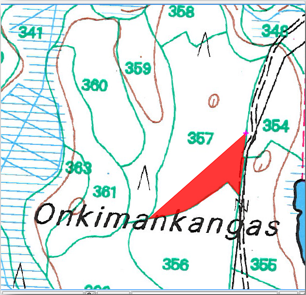
1. Comienza a digitalizar la masa 358 en una de las esquinas comunes con la masa 357.

2. Continue normally until you get to the other common corner for both stands.

3. Finalmente, digitalize alguns pontos dentro do polígono 357 assegurando-se que a borda comum não sofre interseção. Veja a imagem abaixo a esquerda.

4. Haz clic derecho para terminar de editar la masa forestal 358.

5. Enter the ID as 358.

6. Click OK. Your new polygon should have a common border with the stand 357 as you can see in the image below.

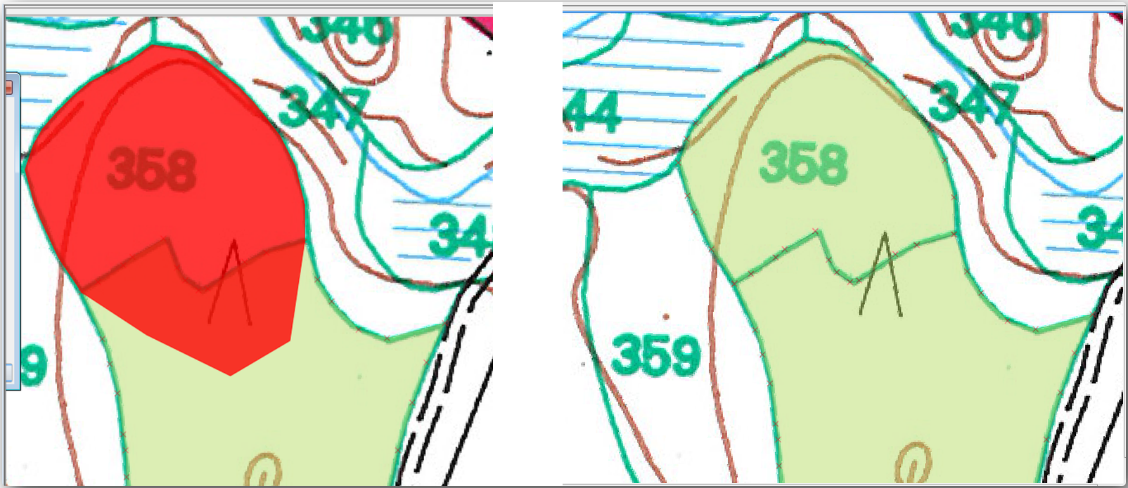
The part of the polygon that was overlapping the existing polygon has been automatically trimmed and you are left with a common border - as you intended it to be.

14.3.5. Try Yourself Terminando la Digitalización de las Masas Forestales

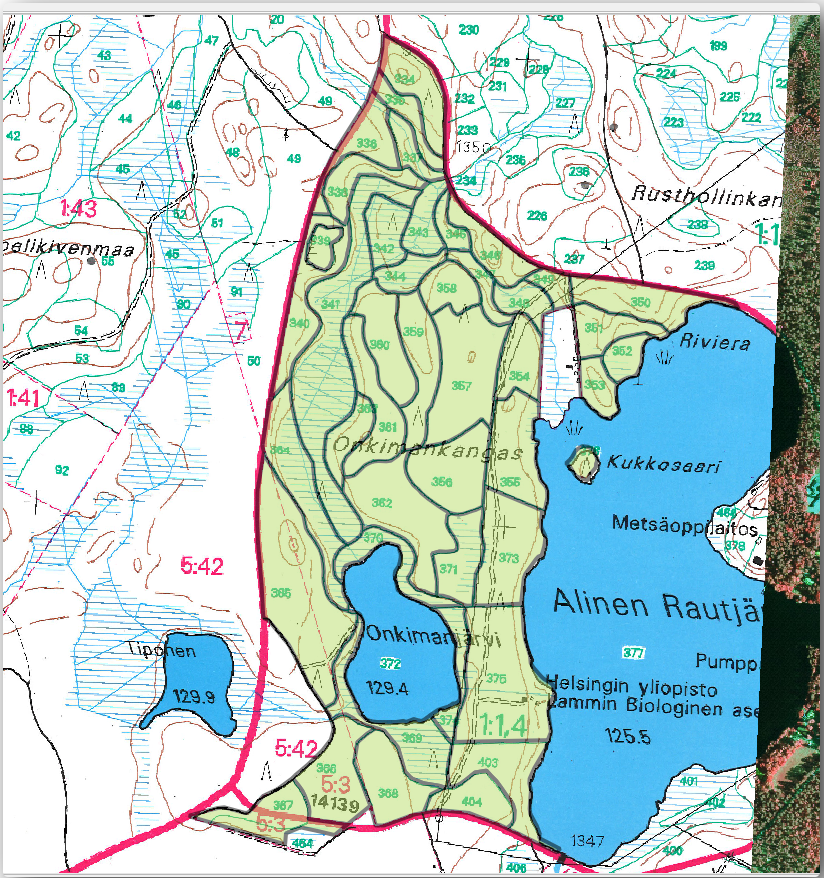
Ahora tienes dos masas forestales diferentes preparadas. Y una buena idea de cómo proceder. Continúa digitalizando por tu cuenta hasta que hayas digitalizado todas las masas forestales que estén limitadas por la calle principal y el lago.

Puede parecer mucho trabajo, pero pronto te acostumbrarás a digitalizar las masas forestales. Debería llevarte unos 15 minutos.

Durante a digitalização você pode precisar editar ou deletar nós, separar ou juntar polígonos. Você aprendeu sobre as ferramentas necessárias em Lesson: Topología de los Elementos, agora provavelmente é um bom momento para voltar a lê-lo.

Recuerda que tener activa la Enable topological editing, te permite mover nodos comunes a dos polígonos para que el borde común sea editado al mismo tiempo para ambos polígonos.

Tu resultado se parecerá a esto:

14.3.6. Follow Along: Añadiendo Datos a las Masas Forestales

Es posible que los datos de inventario forestal que tienes en tu mapa también estén escritos en papel. En ese caso, primero tendrías que haber escrito los datos en un archivo de texto o una hoja de cálculo. Para este ejercicio, la información del inventario para 1994 (el mismo inventario que el mapa) está listo como un archivo de texto separado por comas (csv).

1. Open the rautjarvi_1994.csv file from the exercise_data\forestry directory in a text editor and note that the inventory data file has an attribute called ID that has the numbers of the forest stands. Those numbers are the same as the forest stands ids you have entered for your polygons and can be used to link the data from the text file to your vector file. You can see the metadata for this inventory data in the file rautjarvi_1994_legend.txt in the same folder.

2. Now add this file into the project:

   1. Use the ^{Add Delimited Text Layer} tool. This is accessed via Layer ► Add Layer ► Add Delimited Text Layer….

   2. Set details in the dialog as follows:

      

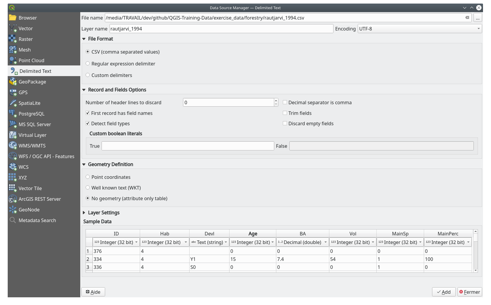
   3. Press Add to load the formatted csv file in the project.

3. To link the data from the .csv file with the digitized polygons, create a join between the two layers:

   1. Open the Layer Properties for the forest_stands layer.

   2. Ve a la pestaña Joins.

   3. Click ^{Add new join} on the bottom of the dialog box.

   4. Select rautjarvi_1994.csv as the Join layer

   5. Set the Join field to ID

   6. Set the Target field to ID

   7. Haz clic en OK dos veces.

The data from the text file should be now linked to your vector file. To see what has happened, select the forest_stands layer and use ^{Open Attribute Table}. You can see that all the attributes from the inventory data file are now linked to your digitized vector layer.

You will see that the field names are prefixed with rautjarvi_1994_. To change this:

1. Open the Layer Properties for the forest_stands layer.

2. Ve a la pestaña Joins.

3. Select Join Layer rautjarvi_1994

4. Click the ^{Edit selected join} button to enable editing

5. Under Custom field name prefix remove the prefix name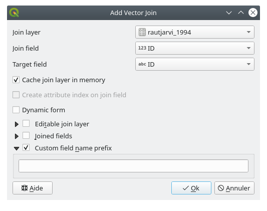

   

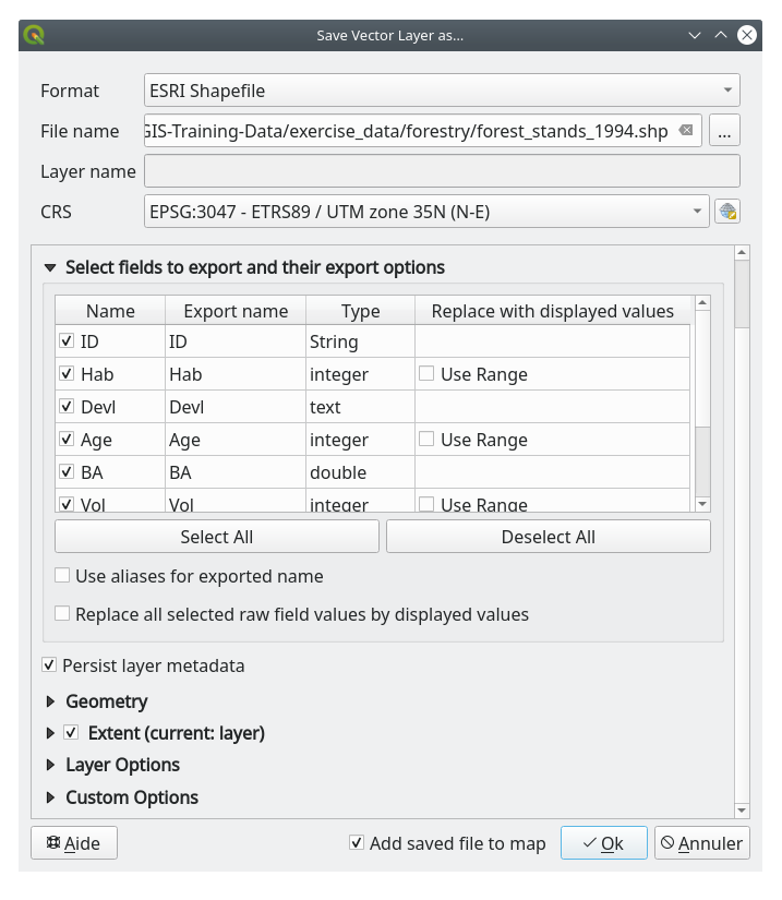
The data from the .csv file is just linked to your vector file. To make this link permanent, so that the data is actually recorded to the vector file you need to save the forest_stands layer as a new vector file. To do this:

1. Right click on forest_stands layer

2. Choose Export ► Save Features As…

3. Set Format to ESRI Shapefile

4. Set file name to forest_stands_1994.shp under the forestry folder

5. To include the new file as a layer in the project, check Add saved file to map

14.3.7. Try Yourself Adding Area and Perimeter

To finish gathering the information related to these forest stands, you might calculate the area and the perimeter of the stands. You calculated areas for polygons in Lesson: Exercício Suplementar. Go back to that lesson if you need to and calculate the areas for the forest stands. Name the new attribute Area and make sure that the values calculated are in hectares. You could also do the same for the perimeter.

Now your forest_stands_1994 layer is ready and packed with all the available information.

Save your project to keep the current map layers in case you need to come back later to it.

14.3.8. In Conclusion

Ha llevado unos pocos clics de ratón pero ahora tienes tus viejos datos de inventario en formato digital y listos para usar en QGIS.

14.3.9. What’s Next?

Podrías empezar haciendo diferentes análisis con tu nueva marca de conjuntos de datos, pero puede que estés más interesado en relizar análisis en un conjunto de datos más actualizado. El tema de la siguiente lección será la creación de masas forestales utilizando fotos aéreas actuales y la adición de información relevante a tu conjunto de datos.