14.3. Lesson: Digitizing Forest Stands

Unless you are going to use your georeferenced map as a simple background image, the next natural step is to digitize elements from it. You have already done so in the exercises about creating vector data in Lesson: Creating a New Vector Dataset, when you digitized the school fields. In this lesson, you are going to digitize the forest stands‘ borders that appear in the map as green lines but instead of doing it using an aerial image, you will use your georeferenced map.

The goal for this lesson: Learn a technique to help the digitizing task, digitizing forest stands and finally adding the inventory data to them.

14.3.1. Follow Along: Extracting the Forest Stands Borders

Open your map_digitizing.qgs project in QGIS, that you saved from the previous lesson.

Once you have scanned and georeferenced your map you could start to digitize directly by looking at the image as a guide. That would most likely be the way to go if the image you are going to digitize from is, for example, an aerial photograph.

If what you are using to digitize is a good map, as it is in our case, it is likely that the information is clearly displayed as lines with different colors for each type of element. Those colors can be relatively easy extracted as individual images using an image processing software like GIMP. Such separate images can be used to assist the digitizing, as you will see below.

The first step will be to use GIMP to obtain an image that contains only the forest stands, that is, all those greenish lines that you could see in the original scanned map:

1. Open GIMP (if you don’t have it installed yet, download it from the internet or ask your teacher).

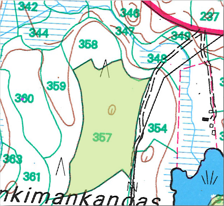
2. Open the original map image, File ► Open, rautjarvi_map.tif in the exercise_data/forestry folder. Note that the forest stands are represented as green lines (with the number of the stand also in green inside each polygon).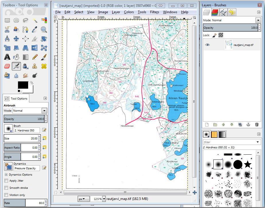

   

   
   

3. Now you can select the pixels in the image that are making up the forest stands‘ borders (the greenish pixels):

   1. Open the tool Select ► By color.

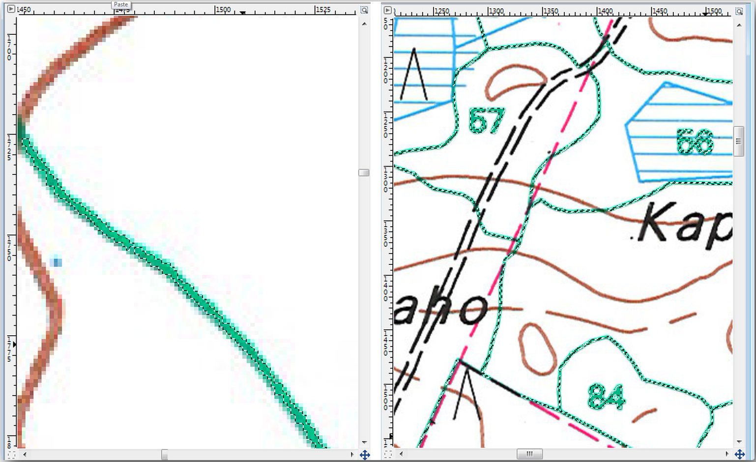
   2. With the tool active, zoom into the image (Ctrl + mouse wheel) so that a forest stand line is close enough to differentiate the pixels forming the line. See the left image below.

   3. Click and drag the mouse cursor in the middle of the line so that the tool will collect several pixel color values.

   4. Release the mouse click and wait a few seconds. The pixels matching the colors collected by the tool will be selected through the whole image.

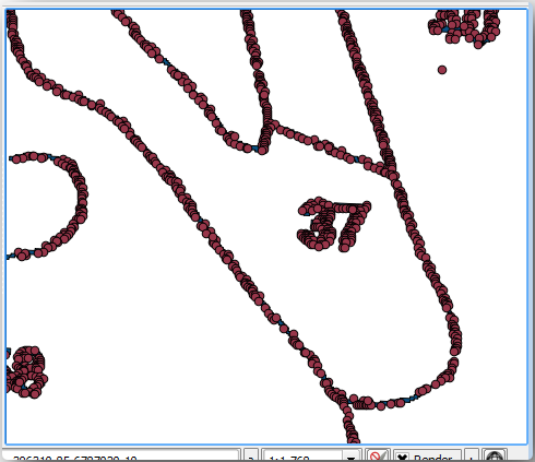
   5. Zoom out to see how the greenish pixels have been selected throughout the image.

   6. If you are not happy with the result, repeat the click and drag operation.

   7. Your pixel selection should look something like the right image below.

   

   
   

4. Once you are done with the selection you need to copy this selection as a new layer and then save it as separate image file:

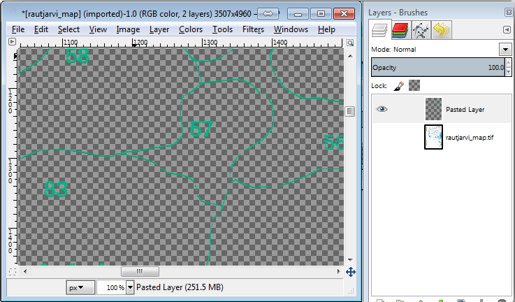
   1. Copy (Ctr+C) the selected pixels.

   2. And paste the pixels directly (Ctr+V), GIMP will display the pasted pixels as a new temporary layer in the Layers - Brushes panel as a Floating Selection (Pasted Layer).

   3. Right click that temporary layer and select To New Layer.

   4. Click the „eye“ icon next to the original image layer to switch it off, so that only the Pasted Layer is visible:

   

   
   

5. Finally, select File ► Export…, set Select File Type (By Extension) as a TIFF image, select the digitizing folder and name it rautjarvi_map_green.tif. Select no compression when asked.

You could do the same process with other elements in the image, for example extracting the black lines that represent roads or the brown ones that represent the terrain‘ contour lines. But for us, the forest stands is enough.

14.3.2. Try Yourself Georeference the Green Pixels Image

As you did in the previous lesson, you need to georeference this new image to be able to use it with the rest of your data.

Note that you don’t need to digitize the ground control points anymore because this image is basically the same image as the original map image, as far as the Georeferencer tool is concerned. Here are some things you should remember:

• This image is also, of course, in KKJ / Finland zone 2 CRS.

• You should use the ground control points you saved, File ► Load GCP points.

• Remember to review the Transformation settings.

• Name the output raster as rautjarvi_green_georef.tif in the digitizing folder.

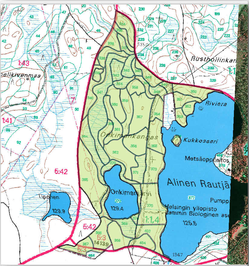
Check that the new raster is fitting nicely with the original map.

14.3.3. Follow Along: Creating Supporting Points for Digitizing

Having in mind the digitizing tools in QGIS, you might already be thinking that it would be helpful to snap to those green pixels while digitizing. That is precisely what you are going to do next create points from those pixels to use them later to help you follow the forest stands‘ borders when digitizing, by using the snapping tools available in QGIS.

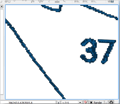
1. Use the Raster ► Conversion ► Polygonize (Raster to Vector) tool to vectorize your green lines to polygons. If you don’t remember how, you can review it in Lesson: Raster to Vector Conversion.

2. Save as rautjarvi_green_polygon.shp inside the digitizing folder.

3. Zoom in and see what the polygons look like. You will get something like this:

   

   
   

4. Next option to get points out of those polygons is to get their centroids:

   1. Open Vector ► Geometry Tools ► Centroids….

   2. Set Input Layer to rautjarvi_green_polygon (the polygon layer you have just created)

   3. Set Centroids output to green_centroids.shp file within the folder digitizing

   4. Check Open output file after running algorithm

   5. Press Run. This will calculate the centroids for the polygons as a new layer and add it to the project.

   

   
   

5. Now you can remove the rautjarvi_green_polygon layer from the TOC.

6. Change the symbology of the centroids layer as follows:

   1. Open the Layer Properties for green_centroids.

   2. Go to the Symbology tab.

   3. Set Size to 1.00 and choose Map Units

It is not necessary to differentiate points from each other, you just need them to be there for the snapping tools to use them. You can use those points now to follow the original lines much easily than without them.

14.3.4. Follow Along: Digitize the Forest Stands

Now you are ready to start with the actual digitizing work. You would start by creating a vector file of polygon type, but for this exercise, there is a shapefile with part of the area of interest already digitized. You will just finish digitizing the half of the forest stands that are left between the main roads (wide pink lines) and the lake:

1. Go to the digitizing folder using your file manager browser.

2. Drag and drop the forest_stands.shp vector file to your map.

3. Change the new layer’s symbology so that it will be easier to see the polygons that have already been digitized.

   1. Set Fill color to green - and change the Opacity to 50%.

   2. Select Simple Fill and set Stroke width to 1.00 mm.

Now, if you remember past modules, we have to set up and activate the snapping options:

1. Go to Project ► Snapping options…

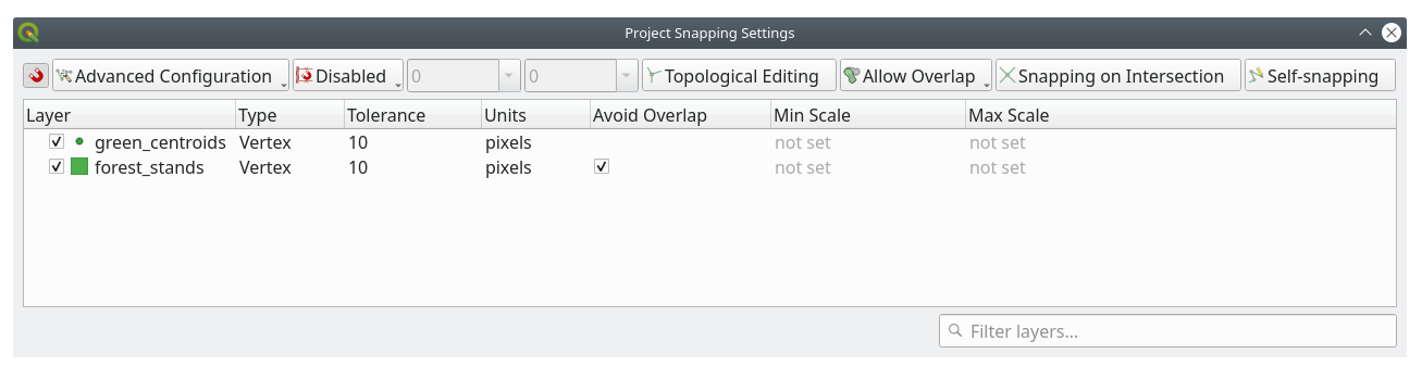
2. Press ^{Enable Snapping} and select Advanced Configuration

3. Check the green_centroids and forest_stands layers

4. Set Type for each layer to Vertex

5. Set Tolerance for each layer to 10

6. Set Units for each layer to pixels

7. Check Avoid Overlap for the forest_stands layer

8. Press Topological editing

9. Choose Follow Advanced Configuration

10. Close the pop-up

    

    With these snapping settings, whenever you are digitizing and get close enough to one of the points in the centroids layer or any vertex of your digitized polygons, a pink square will appear on the point that will be snapped to.

11. Finally, turn off the visibility of all the layers except forest_stands and rautjarvi_georef. Make sure that the map image has not transparency any more.

A few important things to note before you start digitizing:

• Don’t try to be too accurate with the digitizing of the borders.

• If a border is a straight line, digitize it with just two nodes. In general, digitize using as few nodes as possible.

• Zoom in to close ranges only if you feel that you need to be accurate, for example, at some corners or when you want a polygon to connect with another polygon at a certain node.

• Use the mouse’s middle button to zoom in/out and to pan as you digitize.

• Digitize only one polygon at a time.

• After digitizing one polygon, write the forest stand id that you can see from the map.

Now you can start digitizing:

1. Locate the forest stand number 357 in the map window.

2. Select the forest_stands layer.

3. Click the ^{Toggle Editing} button to enable editing

4. Select ^{Add Polygon Feature} tool.

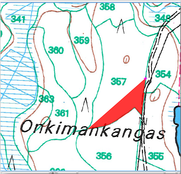
5. Start digitizing the stand 357 by connecting some of the dots. Note the pink crosses indicating the snapping.

When you are done:

1. Right click to end digitizing that polygon.

2. Enter the forest stand ID within the form (in this case 357).

3. Click OK.

If a form did not appear when you finished digitizing the polygon, go to Settings ► Options ► Digitizing and make sure that the Suppress attribute form pop-up after feature creation is not checked.

Your digitized polygon will look like this:

Now for the second polygon, pick up the stand number 358. Make sure that Avoid Overlap is checked for the forest_stands layer (as shown above). This option ensures polygons do not overlap. So, if you digitize over an existing polygon, the new polygon will be trimmed to meet the border of the existing polygons. You can use this option to automatically obtain a common border.

1. Begin digitizing the stand 358 at one of the common corners with the stand 357.

2. Continue normally until you get to the other common corner for both stands.

3. Finally, digitize a few points inside polygon 357 making sure that the common border is not intersected. See left image below.

4. Right click to finish editing the forest stand 358.

5. Enter the ID as 358.

6. Click OK. Your new polygon should have a common border with the stand 357 as you can see in the image below.

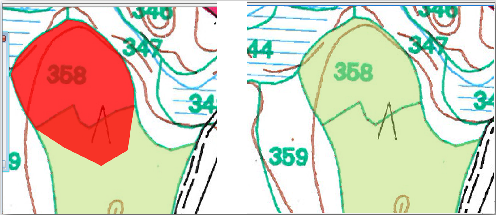
The part of the polygon that was overlapping the existing polygon has been automatically trimmed and you are left with a common border - as you intended it to be.

14.3.5. Try Yourself Finish Digitizing the Forest Stands

Now you have two forest stands ready. And a good idea on how to proceed. Continue digitizing on your own until you have digitized all the forest stands that are limited by the main road and the lake.

It might look like a lot of work, but you will soon get used to digitizing the forest stands. It should take you about 15 minutes.

During the digitizing you might need to edit or delete nodes, split or merge polygons. You learned about the necessary tools in Lesson: Funktionstopologie, now is probably a good moment to go read about them again.

Remember that having Enable topological editing activated, allows you to move nodes common to two polygons so that the common border is edited at the same time for both polygons.

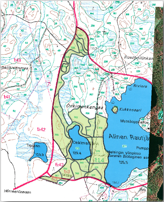
Your result will look like this:

14.3.6. Follow Along: Joining the Forest Stand Data

It is possible that the forest inventory data you have for you map is also written in paper. In that case, you would have to first write that data to a text file or a spreadsheet. For this exercise, the information from the inventory for 1994 (the same inventory as the map) is ready as a comma separated text (csv) file.

1. Open the rautjarvi_1994.csv file from the exercise_data\forestry directory in a text editor and note that the inventory data file has an attribute called ID that has the numbers of the forest stands. Those numbers are the same as the forest stands ids you have entered for your polygons and can be used to link the data from the text file to your vector file. You can see the metadata for this inventory data in the file rautjarvi_1994_legend.txt in the same folder.

2. Now add this file into the project:

   1. Use the ^{Add Delimited Text Layer} tool. This is accessed via Layer ► Add Layer ► Add Delimited Text Layer….

   2. Set details in the dialog as follows:

      

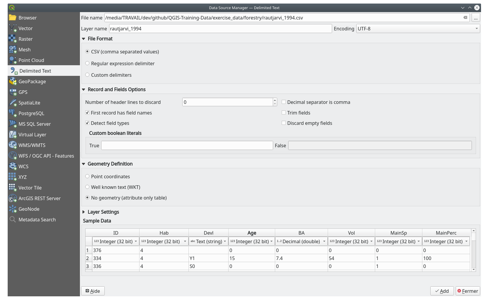
   3. Press Add to load the formatted csv file in the project.

3. To link the data from the .csv file with the digitized polygons, create a join between the two layers:

   1. Open the Layer Properties for the forest_stands layer.

   2. Go to the Joins tab.

   3. Click ^{Add new join} on the bottom of the dialog box.

   4. Select rautjarvi_1994.csv as the Join layer

   5. Set the Join field to ID

   6. Set the Target field to ID

   7. Click OK two times.

The data from the text file should be now linked to your vector file. To see what has happened, select the forest_stands layer and use ^{Open Attribute Table}. You can see that all the attributes from the inventory data file are now linked to your digitized vector layer.

You will see that the field names are prefixed with rautjarvi_1994_. To change this:

1. Open the Layer Properties for the forest_stands layer.

2. Go to the Joins tab.

3. Select Join Layer rautjarvi_1994

4. Click the ^{Edit selected join} button to enable editing

5. Under Custom field name prefix remove the prefix name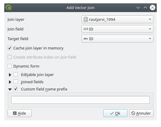

   

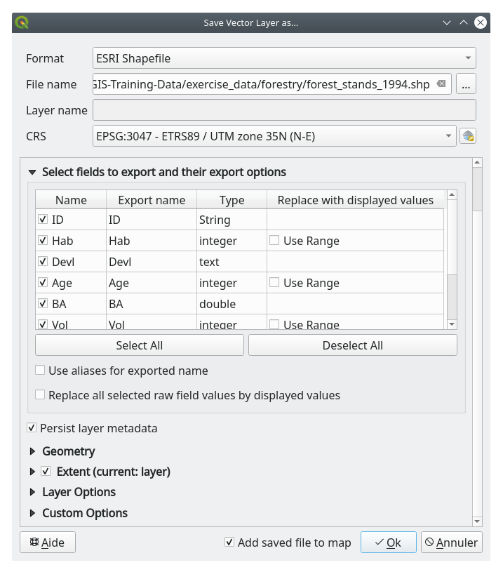
The data from the .csv file is just linked to your vector file. To make this link permanent, so that the data is actually recorded to the vector file you need to save the forest_stands layer as a new vector file. To do this:

1. Right click on forest_stands layer

2. Choose Export ► Save Features As…

3. Set Format to ESRI Shapefile

4. Set file name to forest_stands_1994.shp under the forestry folder

5. To include the new file as a layer in the project, check Add saved file to map

14.3.7. Try Yourself Adding Area and Perimeter

To finish gathering the information related to these forest stands, you might calculate the area and the perimeter of the stands. You calculated areas for polygons in Lesson: Supplementary Exercise. Go back to that lesson if you need to and calculate the areas for the forest stands. Name the new attribute Area and make sure that the values calculated are in hectares. You could also do the same for the perimeter.

Now your forest_stands_1994 layer is ready and packed with all the available information.

Save your project to keep the current map layers in case you need to come back later to it.

14.3.8. In Conclusion

It has taken a few clicks of the mouse but you now have your old inventory data in digital format and ready for use in QGIS.

14.3.9. What’s Next?

You could start doing different analysis with your brand new dataset, but you might be more interested in performing analysis in a dataset more up to date. The topic of the next lesson will be the creation of forest stands using current aerial photos and the addition of some relevant information to your dataset.