9.2. List of functions
The functions, operators and variables available in QGIS are listed below, grouped by categories.
9.2.1. Aggregates Functions
This group contains functions which aggregate values over layers and fields.
Show/hide list of functions
9.2.1.1. aggregate
Returns an aggregate value calculated using features from another layer.
Syntax |
aggregate(layer, aggregate, expression, [filter], [concatenator:=’’], [order_by]) [] marks optional arguments |
Arguments |
|
Examples |
|
9.2.1.2. array_agg
Returns an array of aggregated values from a field or expression.
Syntax |
array_agg(expression, [group_by], [filter], [order_by]) [] marks optional arguments |
Arguments |
|
Examples |
|
9.2.1.3. collect
Returns the multipart geometry of aggregated geometries from an expression
Syntax |
collect(expression, [group_by], [filter]) [] marks optional arguments |
Arguments |
|
Examples |
|
9.2.1.4. concatenate
Returns all aggregated strings from a field or expression joined by a delimiter.
Syntax |
concatenate(expression, [group_by], [filter], [concatenator:=’’], [order_by]) [] marks optional arguments |
Arguments |
|
Examples |
|
9.2.1.5. concatenate_unique
Returns all unique strings from a field or expression joined by a delimiter.
Syntax |
concatenate_unique(expression, [group_by], [filter], [concatenator:=’’], [order_by]) [] marks optional arguments |
Arguments |
|
Examples |
|
9.2.1.6. count
Returns the count of matching features.
Syntax |
count(expression, [group_by], [filter]) [] marks optional arguments |
Arguments |
|
Examples |
|
9.2.1.7. count_distinct
Returns the count of distinct values.
Syntax |
count_distinct(expression, [group_by], [filter]) [] marks optional arguments |
Arguments |
|
Examples |
|
9.2.1.8. count_missing
Returns the count of missing (NULL) values.
Syntax |
count_missing(expression, [group_by], [filter]) [] marks optional arguments |
Arguments |
|
Examples |
|
9.2.1.9. iqr
Returns the calculated inter quartile range from a field or expression.
Syntax |
iqr(expression, [group_by], [filter]) [] marks optional arguments |
Arguments |
|
Examples |
|
9.2.1.10. majority
Returns the aggregate majority of values (most commonly occurring value) from a field or expression.
Syntax |
majority(expression, [group_by], [filter]) [] marks optional arguments |
Arguments |
|
Examples |
|
9.2.1.11. max_length
Returns the maximum length of strings from a field or expression.
Syntax |
max_length(expression, [group_by], [filter]) [] marks optional arguments |
Arguments |
|
Examples |
|
9.2.1.12. maximum
Returns the aggregate maximum value from a field or expression.
Syntax |
maximum(expression, [group_by], [filter]) [] marks optional arguments |
Arguments |
|
Examples |
|
9.2.1.13. mean
Returns the aggregate mean value from a field or expression.
Syntax |
mean(expression, [group_by], [filter]) [] marks optional arguments |
Arguments |
|
Examples |
|
9.2.1.14. median
Returns the aggregate median value from a field or expression.
Syntax |
median(expression, [group_by], [filter]) [] marks optional arguments |
Arguments |
|
Examples |
|
9.2.1.15. min_length
Returns the minimum length of strings from a field or expression.
Syntax |
min_length(expression, [group_by], [filter]) [] marks optional arguments |
Arguments |
|
Examples |
|
9.2.1.16. minimum
Returns the aggregate minimum value from a field or expression.
Syntax |
minimum(expression, [group_by], [filter]) [] marks optional arguments |
Arguments |
|
Examples |
|
9.2.1.17. minority
Returns the aggregate minority of values (least occurring value) from a field or expression.
Syntax |
minority(expression, [group_by], [filter]) [] marks optional arguments |
Arguments |
|
Examples |
|
9.2.1.18. q1
Returns the calculated first quartile from a field or expression.
Syntax |
q1(expression, [group_by], [filter]) [] marks optional arguments |
Arguments |
|
Examples |
|
9.2.1.19. q3
Returns the calculated third quartile from a field or expression.
Syntax |
q3(expression, [group_by], [filter]) [] marks optional arguments |
Arguments |
|
Examples |
|
9.2.1.20. range
Returns the aggregate range of values (maximum - minimum) from a field or expression.
Syntax |
range(expression, [group_by], [filter]) [] marks optional arguments |
Arguments |
|
Examples |
|
9.2.1.21. relation_aggregate
Returns an aggregate value calculated using all matching child features from a layer relation.
Syntax |
relation_aggregate(relation, aggregate, expression, [concatenator:=’’], [order_by]) [] marks optional arguments |
Arguments |
|
Examples |
|
Further reading: Setting relations between multiple layers
9.2.1.22. stdev
Returns the aggregate standard deviation value from a field or expression.
Syntax |
stdev(expression, [group_by], [filter]) [] marks optional arguments |
Arguments |
|
Examples |
|
9.2.1.23. sum
Returns the aggregate summed value from a field or expression.
Syntax |
sum(expression, [group_by], [filter]) [] marks optional arguments |
Arguments |
|
Examples |
|
9.2.2. Array Functions
This group contains functions to create and manipulate arrays (also known as list data structures). The order of values within the array matters, unlike the ‘map’ data structure, where the order of key-value pairs is irrelevant and values are identified by their keys.
Show/hide list of functions
9.2.2.1. array
Returns an array containing all the values passed as parameter.
Syntax |
array(value1, value2, …) |
Arguments |
|
Examples |
|
9.2.2.2. array_all
Returns TRUE if an array contains all the values of a second array.
Syntax |
array_all(array1, array2) |
Arguments |
|
Examples |
|
9.2.2.3. array_append
Returns an array with the given value added at the end.
Syntax |
array_append(array, value) |
Arguments |
|
Examples |
|
9.2.2.4. array_cat
Returns an array containing all the given arrays concatenated.
Syntax |
array_cat(array1, array2, …) |
Arguments |
|
Examples |
|
9.2.2.5. array_contains
Returns TRUE if an array contains the given value.
Syntax |
array_contains(array, value) |
Arguments |
|
Examples |
|
9.2.2.6. array_count
Counts the number of occurrences of a given value in an array.
Syntax |
array_count(array, value) |
Arguments |
|
Examples |
|
9.2.2.7. array_distinct
Returns an array containing distinct values of the given array.
Syntax |
array_distinct(array) |
Arguments |
|
Examples |
|
9.2.2.8. array_filter
Returns an array with only the items for which the expression evaluates to true.
Syntax |
array_filter(array, expression, [limit:=0]) [] marks optional arguments |
Arguments |
|
Examples |
|
9.2.2.9. array_find
Returns the lowest index (0 for the first one) of a value within an array. Returns -1 if the value is not found.
Syntax |
array_find(array, value) |
Arguments |
|
Examples |
|
9.2.2.10. array_first
Returns the first value of an array.
Syntax |
array_first(array) |
Arguments |
|
Examples |
|
9.2.2.11. array_foreach
Returns an array with the given expression evaluated on each item.
Syntax |
array_foreach(array, expression) |
Arguments |
|
Examples |
|
9.2.2.12. array_get
Returns the Nth value (0 for the first one) or the last -Nth value (-1 for the last one) of an array.
Syntax |
array_get(array, pos) |
Arguments |
|
Examples |
|
Hint
You can also use the index operator ([]) to get a value from an array.
9.2.2.13. array_insert
Returns an array with the given value added at the given position.
Syntax |
array_insert(array, pos, value) |
Arguments |
|
Examples |
|
9.2.2.14. array_intersect
Returns TRUE if at least one element of array1 exists in array2.
Syntax |
array_intersect(array1, array2) |
Arguments |
|
Examples |
|
9.2.2.15. array_last
Returns the last value of an array.
Syntax |
array_last(array) |
Arguments |
|
Examples |
|
9.2.2.16. array_length
Returns the number of elements of an array.
Syntax |
array_length(array) |
Arguments |
|
Examples |
|
9.2.2.17. array_majority
Returns the most common values in an array.
Syntax |
array_majority(array, [option:=’all’]) [] marks optional arguments |
Arguments |
|
Examples |
|
9.2.2.18. array_max
Returns the maximum value of an array.
Syntax |
array_max(array) |
Arguments |
|
Examples |
|
9.2.2.19. array_mean
Returns the mean of arithmetic values in an array. Non numeric values in the array are ignored.
Syntax |
array_mean(array) |
Arguments |
|
Examples |
|
9.2.2.20. array_median
Returns the median of arithmetic values in an array. Non arithmetic values in the array are ignored.
Syntax |
array_median(array) |
Arguments |
|
Examples |
|
9.2.2.21. array_min
Returns the minimum value of an array.
Syntax |
array_min(array) |
Arguments |
|
Examples |
|
9.2.2.22. array_minority
Returns the less common values in an array.
Syntax |
array_minority(array, [option:=’all’]) [] marks optional arguments |
Arguments |
|
Examples |
|
9.2.2.23. array_prepend
Returns an array with the given value added at the beginning.
Syntax |
array_prepend(array, value) |
Arguments |
|
Examples |
|
9.2.2.24. array_prioritize
Returns an array sorted using the ordering specified in another array. Values which are present in the first array but are missing from the second array will be added to the end of the result.
Syntax |
array_prioritize(array, priority) |
Arguments |
|
Examples |
|
9.2.2.25. array_remove_all
Returns an array with all the entries of the given value removed.
Syntax |
array_remove_all(array, value) |
Arguments |
|
Examples |
|
9.2.2.26. array_remove_at
Returns an array with the item at the given index removed. Supports positive (0 for the first element) and negative (the last -Nth value, -1 for the last element) index.
Syntax |
array_remove_at(array, pos) |
Arguments |
|
Examples |
|
9.2.2.27. array_replace
Returns an array with the supplied value, array, or map of values replaced.
Value & array variant
Returns an array with the supplied value or array of values replaced by another value or an array of values.
Syntax |
array_replace(array, before, after) |
Arguments |
|
Examples |
|
Map variant
Returns an array with the supplied map keys replaced by their paired values.
Syntax |
array_replace(array, map) |
Arguments |
|
Examples |
|
Further reading: replace, regexp_replace
9.2.2.28. array_reverse
Returns the given array with array values in reversed order.
Syntax |
array_reverse(array) |
Arguments |
|
Examples |
|
9.2.2.29. array_slice
Returns a portion of the array. The slice is defined by the start_pos and end_pos arguments.
Syntax |
array_slice(array, start_pos, end_pos) |
Arguments |
|
Examples |
|
9.2.2.30. array_sort
Returns the provided array with its elements sorted.
Syntax |
array_sort(array, [ascending:=true]) [] marks optional arguments |
Arguments |
|
Examples |
|
9.2.2.31. array_sum
Returns the sum of arithmetic values in an array. Non numeric values in the array are ignored.
Syntax |
array_sum(array) |
Arguments |
|
Examples |
|
9.2.2.32. array_to_string
Concatenates array elements into a string separated by a delimiter and using optional string for empty values.
Syntax |
array_to_string(array, [delimiter:=’,’], [emptyvalue:=’’]) [] marks optional arguments |
Arguments |
|
Examples |
|
Further reading: string_to_array
9.2.2.33. generate_series
Creates an array containing a sequence of numbers.
Syntax |
generate_series(start, stop, [step:=1]) [] marks optional arguments |
Arguments |
|
Examples |
|
9.2.2.34. geometries_to_array
Splits a geometry into simpler geometries in an array.
Syntax |
geometries_to_array(geometry) |
Arguments |
|
Examples |
|
9.2.2.35. regexp_matches
Returns an array of all strings captured by capturing groups, in the order the groups themselves appear in the supplied regular expression against a string.
Syntax |
regexp_matches(string, regex, [emptyvalue:=’’]) [] marks optional arguments |
Arguments |
|
Examples |
|
Further reading: substr, regexp_substr
9.2.2.36. string_to_array
Splits string into an array using supplied delimiter and optional string for empty values.
Syntax |
string_to_array(string, [delimiter:=’,’], [emptyvalue:=’’]) [] marks optional arguments |
Arguments |
|
Examples |
|
Further reading: array_to_string
9.2.3. Color Functions
This group contains functions for manipulating colors.
Show/hide list of functions
9.2.3.1. color_cmyk
Returns a string representation of a color based on its cyan, magenta, yellow and black components
Syntax |
color_cmyk(cyan, magenta, yellow, black) |
Arguments |
|
Examples |
|
9.2.3.2. color_cmyka
Returns a string representation of a color based on its cyan, magenta, yellow, black and alpha (transparency) components
Syntax |
color_cmyka(cyan, magenta, yellow, black, alpha) |
Arguments |
|
Examples |
|
9.2.3.3. color_cmykf
Returns a color object based on its cyan, magenta, yellow, black and alpha components.
Syntax |
color_cmykf(cyan, magenta, yellow, black, [alpha:=1.0]) [] marks optional arguments |
Arguments |
|
Examples |
|
9.2.3.4. color_grayscale_average
Applies a grayscale filter to a color and returns it. Returned type is the same as color argument, i.e. a color string representation or a color object.
Syntax |
color_grayscale_average(color) |
Arguments |
|
Examples |
|
9.2.3.5. color_hsl
Returns a string representation of a color based on its hue, saturation, and lightness attributes.
Syntax |
color_hsl(hue, saturation, lightness) |
Arguments |
|
Examples |
|
9.2.3.6. color_hsla
Returns a string representation of a color based on its hue, saturation, lightness and alpha (transparency) attributes
Syntax |
color_hsla(hue, saturation, lightness, alpha) |
Arguments |
|
Examples |
|
9.2.3.7. color_hslf
Returns a color object based on its hue, saturation, and lightness attributes.
Syntax |
color_hslf(hue, saturation, lightness, [alpha:=1.0]) [] marks optional arguments |
Arguments |
|
Examples |
|
9.2.3.8. color_hsv
Returns a string representation of a color based on its hue, saturation, and value attributes.
Syntax |
color_hsv(hue, saturation, value) |
Arguments |
|
Examples |
|
9.2.3.9. color_hsva
Returns a string representation of a color based on its hue, saturation, value and alpha (transparency) attributes.
Syntax |
color_hsva(hue, saturation, value, alpha) |
Arguments |
|
Examples |
|
9.2.3.10. color_hsvf
Returns a color object based on its hue, saturation, and value attributes.
Syntax |
color_hsvf(hue, saturation, value, [alpha:=1.0]) [] marks optional arguments |
Arguments |
|
Examples |
|
9.2.3.11. color_mix
Returns a color mixing the red, green, blue, and alpha values of two provided colors based on a given ratio. Returned type is the same as color arguments, i.e. a color string representation or a color object.
Syntax |
color_mix(color1, color2, ratio) |
Arguments |
|
Examples |
|
9.2.3.12. color_mix_rgb
Returns a string representing a color mixing the red, green, blue, and alpha values of two provided colors based on a given ratio.
Syntax |
color_mix_rgb(color1, color2, ratio) |
Arguments |
|
Examples |
|
9.2.3.13. color_part
Returns a specific component from a color string or color object, e.g., the red component or alpha component.
Syntax |
color_part(color, component) |
Arguments |
|
Examples |
|
9.2.3.14. color_rgb
Returns a string representation of a color based on its red, green, and blue components.
Syntax |
color_rgb(red, green, blue) |
Arguments |
|
Examples |
|
9.2.3.15. color_rgba
Returns a string representation of a color based on its red, green, blue, and alpha (transparency) components.
Syntax |
color_rgba(red, green, blue, alpha) |
Arguments |
|
Examples |
|
9.2.3.16. color_rgbf
Returns a color object based on its red, green, blue and alpha components.
Syntax |
color_rgbf(red, green, blue, [alpha:=1.0]) [] marks optional arguments |
Arguments |
|
Examples |
|
9.2.3.17. create_ramp
Returns a gradient ramp from a map of color strings and steps.
Syntax |
create_ramp(map, [discrete:=false]) [] marks optional arguments |
Arguments |
|
Examples |
|
9.2.3.18. darker
Returns a darker (or lighter) color. Returned type is the same as color arguments, i.e. a color string representation or a color object.
Syntax |
darker(color, factor) |
Arguments |
|
Examples |
|
Further reading: lighter
9.2.3.19. lighter
Returns a lighter (or darker) color. Returned type is the same as color arguments, i.e. a color string representation or a color object.
Syntax |
lighter(color, factor) |
Arguments |
|
Examples |
|
Further reading: darker
9.2.3.20. project_color
Returns a color from the project’s color scheme.
Syntax |
project_color(name) |
Arguments |
|
Examples |
|
Further reading: setting project colors
9.2.3.21. project_color_object
Returns a color from the project’s color scheme. Contrary to project_color which returns a color string representation, project_color_object returns a color object.
Syntax |
project_color_object(name) |
Arguments |
|
Examples |
|
9.2.3.22. ramp_color
Returns a string representing a color from a color ramp.
Saved ramp variant
Returns a string representing a color from a saved ramp
Syntax |
ramp_color(ramp_name, value) |
Arguments |
|
Examples |
|
Note
The color ramps available vary between QGIS installations. This function may not give the expected results if you move your QGIS project between installations.
Expression-created ramp variant
Returns a string representing a color from an expression-created ramp
Syntax |
ramp_color(ramp, value) |
Arguments |
|
Examples |
|
Further reading: Setting a Color Ramp, The color ramp drop-down shortcut
9.2.3.23. ramp_color_object
Returns a color object from a color ramp. Contrary to ramp_color which returns a color string representation, ramp_color_object returns a color object.
Saved ramp variant
Returns a color object from a saved ramp
Syntax |
ramp_color_object(ramp_name, value) |
Arguments |
|
Examples |
|
Note
The color ramps available vary between QGIS installations. This function may not give the expected results if you move your QGIS project between installations.
Expression-created ramp variant
Returns a color object from an expression-created ramp
Syntax |
ramp_color_object(ramp, value) |
Arguments |
|
Examples |
|
9.2.3.24. set_color_part
Sets a specific color component for a color string or a color object, e.g., the red component or alpha component.
Syntax |
set_color_part(color, component, value) |
Arguments |
|
Examples |
|
9.2.4. Conditional Functions
This group contains functions to handle conditional checks in expressions.
Show/hide list of functions
9.2.4.1. CASE
CASE is used to evaluate a series of conditions and return a result for the first condition met. The conditions are evaluated sequentially, and if a condition is true, the evaluation stops, and the corresponding result is returned. If none of the conditions are true, the value in the ELSE clause is returned. Furthermore, if no ELSE clause is set and none of the conditions are met, NULL is returned.
CASE
WHEN condition THEN result
[ …n ]
[ ELSE result ]
END
[ ] marks optional components
Arguments |
|
Examples |
|
9.2.4.2. coalesce
Returns the first non-NULL value from the expression list.
This function can take any number of arguments.
Syntax |
coalesce(expression1, expression2, …) |
Arguments |
|
Examples |
|
9.2.4.3. if
Tests a condition and returns a different result depending on the conditional check.
Syntax |
if(condition, result_when_true, result_when_false) |
Arguments |
|
Examples |
|
9.2.4.4. nullif
Returns a NULL value if value1 equals value2; otherwise it returns value1. This can be used to conditionally substitute values with NULL.
Syntax |
nullif(value1, value2) |
Arguments |
|
Examples |
|
9.2.4.5. regexp_match
Return the first matching position matching a regular expression within an unicode string, or 0 if the substring is not found.
Syntax |
regexp_match(input_string, regex) |
Arguments |
|
Examples |
|
9.2.4.6. try
Tries an expression and returns its value if error-free. If the expression returns an error, an alternative value will be returned when provided otherwise the function will return NULL.
Syntax |
try(expression, [alternative]) [] marks optional arguments |
Arguments |
|
Examples |
|
9.2.5. Conversions Functions
This group contains functions to convert one data type to another (e.g., string from/to integer, binary from/to string, string to date, …).
Show/hide list of functions
9.2.5.1. convert_timezone
Converts a datetime object to a different timezone.
Syntax |
convert_timezone(datetime, timezone) |
Arguments |
|
Examples |
|
9.2.5.2. extract_degrees
Extracts the integer number of degrees from a decimal degrees value. The minutes and seconds components are ignored. The extracted degrees values will be truncated towards zero (not rounded).
Syntax |
extract_degrees(value) |
Arguments |
|
Examples |
|
9.2.5.3. extract_minutes
Extracts the integer number of minutes from a decimal degrees value. The degrees and seconds components are ignored. The extracted minutes values will be truncated towards zero (not rounded), and will always be a positive value.
Syntax |
extract_minutes(value) |
Arguments |
|
Examples |
|
9.2.5.4. extract_seconds
Extracts the decimal number of seconds from a decimal degrees value. The degrees and minutes components are ignored. The extracted seconds value will always be a positive value.
Syntax |
extract_seconds(value) |
Arguments |
|
Examples |
|
9.2.5.5. from_base64
Decodes a string in the Base64 encoding into a binary value.
Syntax |
from_base64(string) |
Arguments |
|
Examples |
|
9.2.5.6. get_timezone
Returns the timezone object associated with a datetime value.
Syntax |
get_timezone(datetime) |
Arguments |
|
Examples |
|
9.2.5.7. hash
Creates a hash from a string with a given method. One byte (8 bits) is represented with two hex ‘’digits’’, so ‘md4’ (16 bytes) produces a 16 * 2 = 32 character long hex string and ‘keccak_512’ (64 bytes) produces a 64 * 2 = 128 character long hex string.
Syntax |
hash(string, method) |
Arguments |
|
Examples |
|
9.2.5.8. md5
Creates a md5 hash from a string.
Syntax |
md5(string) |
Arguments |
|
Examples |
|
9.2.5.9. set_timezone
Sets the timezone object associated with a datetime value, without changing the date or time components. This function can be used to replace the timezone for a datetime.
Syntax |
set_timezone(datetime, timezone) |
Arguments |
|
Examples |
|
9.2.5.10. sha256
Creates a sha256 hash from a string.
Syntax |
sha256(string) |
Arguments |
|
Examples |
|
9.2.5.11. timezone_from_id
Creates a timezone object from a string ID (from the IANA timezone database). The ID must be one of the available system IDs or a valid UTC-with-offset ID.
Syntax |
timezone_from_id(id) |
Arguments |
|
Examples |
|
9.2.5.12. timezone_id
Returns the ID string for a timezone object, using IDs from the IANA timezone database.
Syntax |
timezone_id(timezone) |
Arguments |
|
Examples |
|
9.2.5.13. to_base64
Encodes a binary value into a string, using the Base64 encoding.
Syntax |
to_base64(value) |
Arguments |
|
Examples |
|
9.2.5.14. to_bool
Converts a given value to a boolean. The function will return false if the value is NULL, an empty string, an empty list, or 0.
Syntax |
to_bool(value) |
Arguments |
|
Examples |
|
9.2.5.15. to_date
Converts a string into a date object. An optional format string can be provided to parse the string; see QDate::fromString or the documentation of the format_date function for additional documentation on the format. By default the current QGIS user locale is used.
Syntax |
to_date(string, [format], [language]) [] marks optional arguments |
Arguments |
|
Examples |
|
Further reading: format_date
9.2.5.16. to_datetime
Converts a string into a datetime object. An optional format string can be provided to parse the string; see QDate::fromString, QTime::fromString or the documentation of the format_date function for additional documentation on the format. By default the current QGIS user locale is used.
Syntax |
to_datetime(string, [format], [language]) [] marks optional arguments |
Arguments |
|
Examples |
|
Further reading: format_date
9.2.5.17. to_decimal
Converts a degree, minute, second coordinate to its decimal equivalent.
Syntax |
to_decimal(value) |
Arguments |
|
Examples |
|
9.2.5.18. to_dm
Converts a coordinate to degree, minute.
Syntax |
to_dm(coordinate, axis, precision, [formatting:=NULL]) [] marks optional arguments |
Arguments |
|
Examples |
|
9.2.5.19. to_dms
Converts a coordinate to degree, minute, second.
Syntax |
to_dms(coordinate, axis, precision, [formatting:=NULL]) [] marks optional arguments |
Arguments |
|
Examples |
|
9.2.5.20. to_int
Converts a string to integer number. If a value cannot be converted to integer the expression is invalid (e.g ‘123asd’ is invalid).
Syntax |
to_int(string) |
Arguments |
|
Examples |
|
9.2.5.21. to_interval
Converts a string to an interval type. Can be used to take days, hours, month, etc of a date.
Syntax |
to_interval(string) |
Arguments |
|
Examples |
|
9.2.5.22. to_real
Converts a string to a real number. If a value cannot be converted to real the expression is invalid (e.g ‘123.56asd’ is invalid). Numbers are rounded after saving changes if the precision is smaller than the result of the conversion.
Syntax |
to_real(string) |
Arguments |
|
Examples |
|
9.2.5.23. to_string
Converts a number to string. The conversion is not locale-aware, see ‘format_number’ for a locale-aware alternative.
Syntax |
to_string(number) |
Arguments |
|
Examples |
|
Further reading: format_number
9.2.5.24. to_time
Converts a string into a time object. An optional format string can be provided to parse the string; see QTime::fromString for additional documentation on the format.
Syntax |
to_time(string, [format], [language]) [] marks optional arguments |
Arguments |
|
Examples |
|
Further reading: format_date
9.2.6. CRS Functions
This group contains functions to operate on coordinate reference system objects.
Show/hide list of functions
9.2.6.1. crs_from_text
Creates a coordinate reference system from a string definition. The string can represent an authority ID, a WKT definition, or a PROJ string definition of the CRS.
Syntax |
crs_from_text(definition) |
Arguments |
|
Examples |
|
9.2.6.2. crs_to_authid
Returns the authority ID string for a coordinate reference system.
Syntax |
crs_to_authid(crs) |
Arguments |
|
Examples |
|
9.2.7. Custom Functions
This group contains functions created by the user. See Function Editor for more details.
9.2.8. Date and Time Functions
This group contains functions for handling date and time data. This group shares several functions with the Conversions Functions (to_date, to_time, to_datetime, to_interval) and String Functions (format_date) groups.
Note
Storing date, datetime and intervals on fields
The ability to store date, time and datetime values directly on fields depends on the data source’s provider (e.g., Shapefile accepts date format, but not datetime or time format). The following are some suggestions to overcome this limitation:
date, datetime and time can be converted and stored in text type fields using the format_date() function.
Intervals can be stored in integer or decimal type fields after using one of the date extraction functions (e.g., day() to get the interval expressed in days)
Show/hide list of functions
9.2.8.1. age
Returns the difference between two dates or datetimes.
The difference is returned as an Interval and needs to be used with one of the following functions in order to extract useful information:
yearmonthweekdayhourminutesecond
Syntax |
age(datetime1, datetime2) |
Arguments |
|
Examples |
|
9.2.8.2. convert_timezone
Converts a datetime object to a different timezone.
Syntax |
convert_timezone(datetime, timezone) |
Arguments |
|
Examples |
|
9.2.8.3. datetime_from_epoch
Returns a datetime whose date and time are the number of milliseconds, msecs, that have passed since 1970-01-01T00:00:00.000, Coordinated Universal Time (Qt.UTC), and converted to Qt.LocalTime.
Syntax |
datetime_from_epoch(int) |
Arguments |
|
Examples |
|
9.2.8.4. day
Extracts the day from a date, or the number of days from an interval.
Date variant
Extracts the day from a date or datetime.
Syntax |
day(date) |
Arguments |
|
Examples |
|
Interval variant
Calculates the length in days of an interval.
Syntax |
day(interval) |
Arguments |
|
Examples |
|
9.2.8.5. day_of_week
Returns the day of the week for a specified date or datetime. The returned value ranges from 0 to 6, where 0 corresponds to a Sunday and 6 to a Saturday.
Syntax |
day_of_week(date) |
Arguments |
|
Examples |
|
9.2.8.6. epoch
Returns the interval in milliseconds between the unix epoch and a given date value.
Syntax |
epoch(date) |
Arguments |
|
Examples |
|
9.2.8.7. format_date
Formats a date type or string into a custom string format. Uses Qt date/time format strings. See QDateTime::toString.
Syntax |
format_date(datetime, format, [language]) [] marks optional arguments |
||||||||||||||||||||||||||||||||||||||||||||||||
Arguments |
|
||||||||||||||||||||||||||||||||||||||||||||||||
Examples |
|
9.2.8.8. get_timezone
Returns the timezone object associated with a datetime value.
Syntax |
get_timezone(datetime) |
Arguments |
|
Examples |
|
9.2.8.9. hour
Extracts the hour part from a datetime or time, or the number of hours from an interval.
Time variant
Extracts the hour part from a time or datetime.
Syntax |
hour(datetime) |
Arguments |
|
Examples |
|
Interval variant
Calculates the length in hours of an interval.
Syntax |
hour(interval) |
Arguments |
|
Examples |
|
9.2.8.10. make_date
Creates a date value from year, month and day numbers.
Syntax |
make_date(year, month, day) |
Arguments |
|
Examples |
|
9.2.8.11. make_datetime
Creates a datetime value from year, month, day, hour, minute and second numbers.
Syntax |
make_datetime(year, month, day, hour, minute, second) |
Arguments |
|
Examples |
|
9.2.8.12. make_interval
Creates an interval value from year, month, weeks, days, hours, minute and seconds values.
Syntax |
make_interval([years:=0], [months:=0], [weeks:=0], [days:=0], [hours:=0], [minutes:=0], [seconds:=0]) [] marks optional arguments |
Arguments |
|
Examples |
|
9.2.8.13. make_time
Creates a time value from hour, minute and second numbers.
Syntax |
make_time(hour, minute, second) |
Arguments |
|
Examples |
|
9.2.8.14. minute
Extracts the minutes part from a datetime or time, or the number of minutes from an interval.
Time variant
Extracts the minutes part from a time or datetime.
Syntax |
minute(datetime) |
Arguments |
|
Examples |
|
Interval variant
Calculates the length in minutes of an interval.
Syntax |
minute(interval) |
Arguments |
|
Examples |
|
9.2.8.15. month
Extracts the month part from a date, or the number of months from an interval.
Date variant
Extracts the month part from a date or datetime.
Syntax |
month(date) |
Arguments |
|
Examples |
|
Interval variant
Calculates the length in months of an interval.
Syntax |
month(interval) |
Arguments |
|
Examples |
|
9.2.8.16. now
Returns the current date and time. The function is static and will return consistent results while evaluating. The time returned is the time when the expression is prepared.
Syntax |
now() |
Examples |
|
9.2.8.17. second
Extracts the seconds part from a datetime or time, or the number of seconds from an interval.
Time variant
Extracts the seconds part from a time or datetime.
Syntax |
second(datetime) |
Arguments |
|
Examples |
|
Interval variant
Calculates the length in seconds of an interval.
Syntax |
second(interval) |
Arguments |
|
Examples |
|
9.2.8.18. set_timezone
Sets the timezone object associated with a datetime value, without changing the date or time components. This function can be used to replace the timezone for a datetime.
Syntax |
set_timezone(datetime, timezone) |
Arguments |
|
Examples |
|
9.2.8.19. timezone_from_id
Creates a timezone object from a string ID (from the IANA timezone database). The ID must be one of the available system IDs or a valid UTC-with-offset ID.
Syntax |
timezone_from_id(id) |
Arguments |
|
Examples |
|
9.2.8.20. timezone_id
Returns the ID string for a timezone object, using IDs from the IANA timezone database.
Syntax |
timezone_id(timezone) |
Arguments |
|
Examples |
|
9.2.8.21. to_date
Converts a string into a date object. An optional format string can be provided to parse the string; see QDate::fromString or the documentation of the format_date function for additional documentation on the format. By default the current QGIS user locale is used.
Syntax |
to_date(string, [format], [language]) [] marks optional arguments |
Arguments |
|
Examples |
|
Further reading: format_date
9.2.8.22. to_datetime
Converts a string into a datetime object. An optional format string can be provided to parse the string; see QDate::fromString, QTime::fromString or the documentation of the format_date function for additional documentation on the format. By default the current QGIS user locale is used.
Syntax |
to_datetime(string, [format], [language]) [] marks optional arguments |
Arguments |
|
Examples |
|
Further reading: format_date
9.2.8.23. to_interval
Converts a string to an interval type. Can be used to take days, hours, month, etc of a date.
Syntax |
to_interval(string) |
Arguments |
|
Examples |
|
9.2.8.24. to_time
Converts a string into a time object. An optional format string can be provided to parse the string; see QTime::fromString for additional documentation on the format.
Syntax |
to_time(string, [format], [language]) [] marks optional arguments |
Arguments |
|
Examples |
|
Further reading: format_date
9.2.8.25. week
Extracts the week number from a date, or the number of weeks from an interval.
Date variant
Extracts the week number from a date or datetime.
Syntax |
week(date) |
Arguments |
|
Examples |
|
Interval variant
Calculates the length in weeks of an interval.
Syntax |
week(interval) |
Arguments |
|
Examples |
|
9.2.8.26. year
Extracts the year part from a date, or the number of years from an interval.
Date variant
Extracts the year part from a date or datetime.
Syntax |
year(date) |
Arguments |
|
Examples |
|
Interval variant
Calculates the length in years of an interval.
Syntax |
year(interval) |
Arguments |
|
Examples |
|
Some examples:
Besides these functions, subtracting dates, datetimes or times using the
- (minus) operator will return an interval.
Adding or subtracting an interval to dates, datetimes or times, using the
+ (plus) and - (minus) operators, will return a datetime.
Get the number of days until QGIS 3.0 release:
to_date('2017-09-29') - to_date(now())
-- Returns <interval: 203 days>
The same with time:
to_datetime('2017-09-29 12:00:00') - now()
-- Returns <interval: 202.49 days>
Get the datetime of 100 days from now:
now() + to_interval('100 days')
-- Returns <datetime: 2017-06-18 01:00:00>
9.2.9. Fields and Values
Contains a list of fields from the active layer, and special values. Fields list includes the ones stored in the dataset, virtual and auxiliary ones as well as from joins.
Double-click a field name to have it added to your expression. You can also type the field name (preferably inside double quotes) or its alias.
To retrieve fields values to use in an expression, select the appropriate field and, in the shown widget, choose between 10 Samples and All Unique. Requested values are then displayed and you can use the Search box at the top of the list to filter the result. Sample values can also be accessed via right-clicking on a field.
To add a value to the expression you are writing, double-click on it in the list. If the value is of a string type, it should be simple quoted, otherwise no quote is needed.
Show/hide list of functions
9.2.9.1. NULL
Equates to a NULL value.
Syntax |
NULL |
Examples |
|
Note
To test for NULL use an IS NULL or IS NOT NULL expression.
9.2.10. Files and Paths Functions
This group contains functions which manipulate file and path names.
Show/hide list of functions
9.2.10.1. base_file_name
Returns the base name of the file without the directory or file suffix.
Syntax |
base_file_name(path) |
Arguments |
|
Examples |
|
9.2.10.2. exif
Retrieves exif tag values from an image file.
Syntax |
exif(path, [tag]) [] marks optional arguments |
Arguments |
|
Examples |
|
9.2.10.3. file_exists
Returns TRUE if a file path exists.
Syntax |
file_exists(path) |
Arguments |
|
Examples |
|
9.2.10.4. file_name
Returns the name of a file (including the file extension), excluding the directory.
Syntax |
file_name(path) |
Arguments |
|
Examples |
|
9.2.10.5. file_path
Returns the directory component of a file path. This does not include the file name.
Syntax |
file_path(path) |
Arguments |
|
Examples |
|
9.2.10.6. file_size
Returns the size (in bytes) of a file.
Syntax |
file_size(path) |
Arguments |
|
Examples |
|
9.2.10.7. file_suffix
Returns the file suffix (extension) from a file path.
Syntax |
file_suffix(path) |
Arguments |
|
Examples |
|
9.2.10.8. is_directory
Returns TRUE if a path corresponds to a directory.
Syntax |
is_directory(path) |
Arguments |
|
Examples |
|
9.2.10.9. is_file
Returns TRUE if a path corresponds to a file.
Syntax |
is_file(path) |
Arguments |
|
Examples |
|
9.2.11. Form Functions
This group contains functions that operate exclusively under the attribute form context. For example, in field’s widgets settings.
Show/hide list of functions
9.2.11.1. current_parent_value
Only usable in an embedded form context, this function returns the current, unsaved value of a field in the parent form currently being edited. This will differ from the parent feature’s actual attribute values for features which are currently being edited or have not yet been added to a parent layer. When used in a value-relation widget filter expression, this function should be wrapped into a ‘coalesce()’ that can retrieve the actual parent feature from the layer when the form is not used in an embedded context.
Syntax |
current_parent_value(field_name) |
Arguments |
|
Examples |
|
9.2.11.2. current_value
Returns the current, unsaved value of a field in the form or table row currently being edited. This will differ from the feature’s actual attribute values for features which are currently being edited or have not yet been added to a layer.
Syntax |
current_value(field_name) |
Arguments |
|
Examples |
|
9.2.12. Fuzzy Matching Functions
This group contains functions for fuzzy comparisons between values.
Show/hide list of functions
9.2.12.1. hamming_distance
Returns the Hamming distance between two strings. This equates to the number of characters at corresponding positions within the input strings where the characters are different. The input strings must be the same length, and the comparison is case-sensitive.
Syntax |
hamming_distance(string1, string2) |
Arguments |
|
Examples |
|
9.2.12.2. levenshtein
Returns the Levenshtein edit distance between two strings. This equates to the minimum number of character edits (insertions, deletions or substitutions) required to change one string to another.
The Levenshtein distance is a measure of the similarity between two strings. Smaller distances mean the strings are more similar, and larger distances indicate more different strings. The distance is case sensitive.
Syntax |
levenshtein(string1, string2) |
Arguments |
|
Examples |
|
9.2.12.3. longest_common_substring
Returns the longest common substring between two strings. This substring is the longest string that is a substring of the two input strings. For example, the longest common substring of “ABABC” and “BABCA” is “BABC”. The substring is case sensitive.
Syntax |
longest_common_substring(string1, string2) |
Arguments |
|
Examples |
|
9.2.12.4. soundex
Returns the Soundex representation of a string. Soundex is a phonetic matching algorithm, so strings with similar sounds should be represented by the same Soundex code.
Syntax |
soundex(string) |
Arguments |
|
Examples |
|
9.2.13. General Functions
This group contains general assorted functions.
Show/hide list of functions
9.2.13.1. env
Gets an environment variable and returns its content as a string. If the variable is not found, NULL will be returned. This is handy to inject system specific configuration like drive letters or path prefixes. Definition of environment variables depends on the operating system, please check with your system administrator or the operating system documentation how this can be set.
Syntax |
env(name) |
Arguments |
|
Examples |
|
9.2.13.2. eval
Evaluates an expression which is passed in a string. Useful to expand dynamic parameters passed as context variables or fields.
Syntax |
eval(expression) |
Arguments |
|
Examples |
|
9.2.13.3. eval_template
Evaluates a template which is passed in a string. Useful to expand dynamic parameters passed as context variables or fields.
Syntax |
eval_template(template) |
Arguments |
|
Examples |
|
9.2.13.4. is_layer_visible
Returns TRUE if a specified layer is visible.
Syntax |
is_layer_visible(layer) |
Arguments |
|
Examples |
|
9.2.13.5. mime_type
Returns the mime type of the binary data.
Syntax |
mime_type(bytes) |
Arguments |
|
Examples |
|
9.2.13.6. var
Returns the value stored within a specified variable.
Syntax |
var(name) |
Arguments |
|
Examples |
|
Further reading: List of default variables
9.2.13.7. with_variable
This function sets a variable for any expression code that will be provided as 3rd argument. This is only useful for complicated expressions, where the same calculated value needs to be used in different places.
Syntax |
with_variable(name, value, expression) |
Arguments |
|
Examples |
|
9.2.14. Geometry Functions
This group contains functions that operate on geometry objects (e.g. buffer, transform, $area).
Show/hide list of functions
9.2.14.1. affine_transform
Returns the geometry after an affine transformation. Calculations are in the Spatial Reference System of this geometry. The operations are performed in a scale, rotation, translation order. If there is a Z or M offset but the coordinate is not present in the geometry, it will be added.
Syntax |
affine_transform(geometry, delta_x, delta_y, rotation_z, scale_x, scale_y, [delta_z:=0], [delta_m:=0], [scale_z:=1], [scale_m:=1]) [] marks optional arguments |
Arguments |
|
Examples |
|
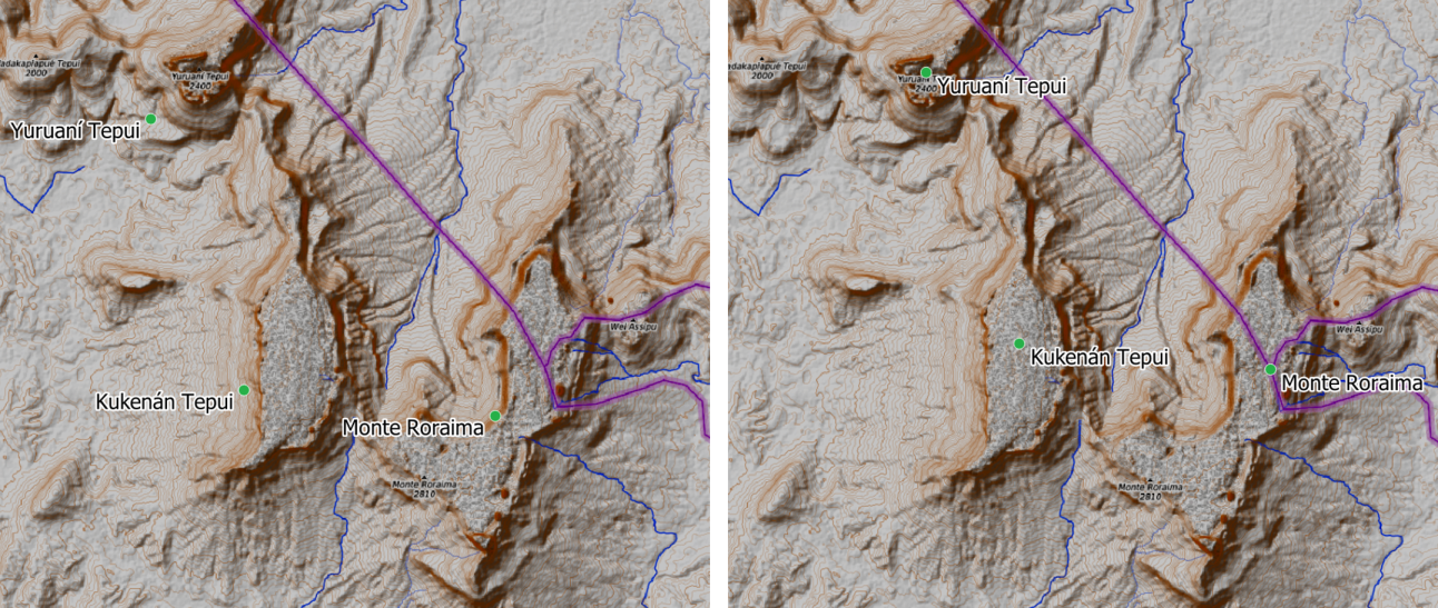
Fig. 9.4 Vector point layer (green dots) before (left), and after (right) an affine transformation (translation).
9.2.14.2. angle_at_vertex
Returns the bisector angle (average angle) to the geometry for a specified vertex on a linestring geometry. Angles are in degrees clockwise from north.
Syntax |
angle_at_vertex(geometry, vertex) |
Arguments |
|
Examples |
|
9.2.14.3. apply_dash_pattern
Applies a dash pattern to a geometry, returning a MultiLineString geometry which is the input geometry stroked along each line/ring with the specified pattern.
Syntax |
apply_dash_pattern(geometry, pattern, [start_rule:=’no_rule’], [end_rule:=’no_rule’], [adjustment:=’both’], [pattern_offset:=0]) [] marks optional arguments |
Arguments |
|
Examples |
|
9.2.14.4. $area
Returns the area of the current feature. The area calculated by this function respects both the current project’s ellipsoid setting and area unit settings. For example, if an ellipsoid has been set for the project then the calculated area will be ellipsoidal, and if no ellipsoid is set then the calculated area will be planimetric.
Syntax |
$area |
Examples |
|
9.2.14.5. area
Returns the area of a geometry polygon object. Calculations are always planimetric in the Spatial Reference System (SRS) of this geometry, and the units of the returned area will match the units for the SRS. This differs from the calculations performed by the $area function, which will perform ellipsoidal calculations based on the project’s ellipsoid and area unit settings.
Syntax |
area(geometry) |
Arguments |
|
Examples |
|
9.2.14.6. azimuth
Returns the north-based azimuth as the angle in radians measured clockwise from the vertical on point1 to point2.
Syntax |
azimuth(point1, point2) |
Arguments |
|
Examples |
|
9.2.14.7. bearing
Returns the north-based bearing as the angle in radians measured clockwise on the ellipsoid from the vertical on point1 to point2.
Syntax |
bearing(point1, point2, [source_crs], [ellipsoid]) [] marks optional arguments |
Arguments |
|
Examples |
|
9.2.14.8. boundary
Returns the closure of the combinatorial boundary of the geometry (ie the topological boundary of the geometry). For instance, a polygon geometry will have a boundary consisting of the linestrings for each ring in the polygon. Some geometry types do not have a defined boundary, e.g., points or geometry collections, and will return NULL.
Syntax |
boundary(geometry) |
Arguments |
|
Examples |
|
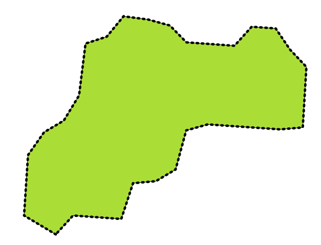
Fig. 9.5 Boundary (black dashed line) of the source polygon layer
Further reading: Boundary algorithm
9.2.14.9. bounds
Returns a geometry which represents the bounding box of an input geometry. Calculations are in the Spatial Reference System of this geometry.
Syntax |
bounds(geometry) |
Arguments |
|
Examples |
|
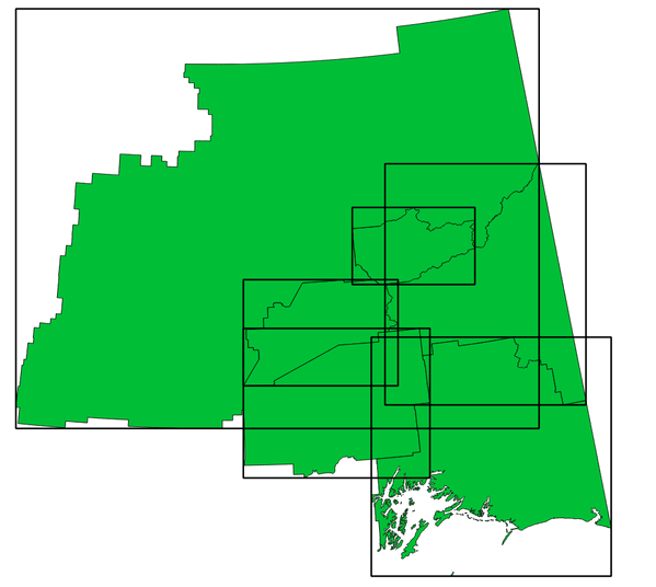
Fig. 9.6 Black lines represent the bounding boxes of each polygon feature
Further reading: Bounding boxes algorithm
9.2.14.10. bounds_height
Returns the height of the bounding box of a geometry. Calculations are in the Spatial Reference System of this geometry.
Syntax |
bounds_height(geometry) |
Arguments |
|
Examples |
|
9.2.14.11. bounds_width
Returns the width of the bounding box of a geometry. Calculations are in the Spatial Reference System of this geometry.
Syntax |
bounds_width(geometry) |
Arguments |
|
Examples |
|
9.2.14.12. buffer
Returns a geometry that represents all points whose distance from this geometry is less than or equal to distance. Calculations are in the Spatial Reference System of this geometry.
Syntax |
buffer(geometry, distance, [segments:=8], [cap:=’round’], [join:=’round’], [miter_limit:=2]) [] marks optional arguments |
Arguments |
|
Examples |
|
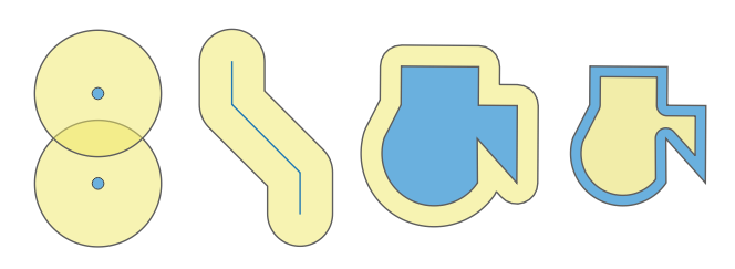
Fig. 9.7 Buffer (in yellow) of points, line, polygon with positive buffer, and polygon with negative buffer
Further reading: Buffer algorithm
9.2.14.13. buffer_by_m
Creates a buffer along a line geometry where the buffer diameter varies according to the m-values at the line vertices.
Syntax |
buffer_by_m(geometry, [segments:=8]) [] marks optional arguments |
Arguments |
|
Examples |
|
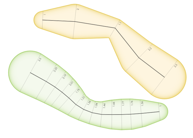
Fig. 9.8 Buffering line features using the m value on the vertices
Further reading: Variable width buffer (by M value) algorithm
9.2.14.14. centroid
Returns the geometric center of a geometry.
Syntax |
centroid(geometry) |
Arguments |
|
Examples |
|
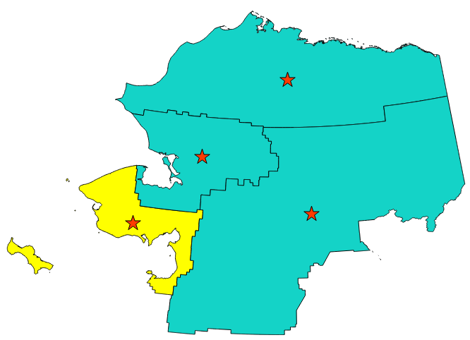
Fig. 9.9 The red stars represent the centroids of the features of the input layer.
Further reading: Centroids algorithm
9.2.14.15. close_line
Returns a closed line string of the input line string by appending the first point to the end of the line, if it is not already closed. If the geometry is not a line string or multi line string then the result will be NULL.
Syntax |
close_line(geometry) |
Arguments |
|
Examples |
|
9.2.14.16. closest_point
Returns the point on geometry1 that is closest to geometry2.
Syntax |
closest_point(geometry1, geometry2) |
Arguments |
|
Examples |
|
9.2.14.17. collect_geometries
Collects a set of geometries into a multi-part geometry object.
List of arguments variant
Geometry parts are specified as separate arguments to the function.
Syntax |
collect_geometries(geometry1, geometry2, …) |
Arguments |
|
Examples |
|
Array variant
Geometry parts are specified as an array of geometry parts.
Syntax |
collect_geometries(array) |
Arguments |
|
Examples |
|
Further reading: Collect geometries algorithm
9.2.14.18. combine
Returns the combination of two geometries.
Syntax |
combine(geometry1, geometry2) |
Arguments |
|
Examples |
|
9.2.14.19. concave_hull
Returns a possibly concave polygon that contains all the points in the geometry
Syntax |
concave_hull(geometry, target_percent, [allow_holes:=false]) [] marks optional arguments |
Arguments |
|
Examples |
|
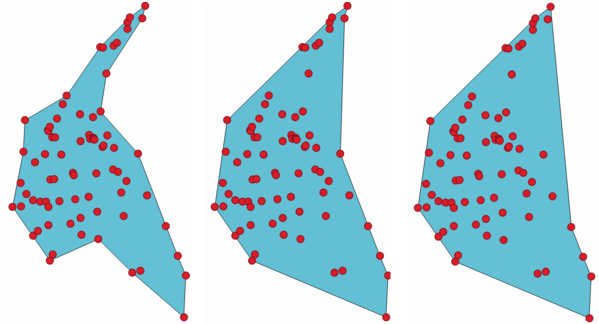
Fig. 9.10 Concave hulls with increasing target_percent parameter
Further reading: convex_hull, Concave hull (by layer) algorithm
9.2.14.20. contains
Tests whether a geometry contains another. Returns TRUE if and only if no points of geometry2 lie in the exterior of geometry1, and at least one point of the interior of geometry2 lies in the interior of geometry1.
Syntax |
contains(geometry1, geometry2) |
Arguments |
|
Examples |
|
Further reading: overlay_contains
9.2.14.21. convex_hull
Returns the convex hull of a geometry. It represents the minimum convex geometry that encloses all geometries within the set.
Syntax |
convex_hull(geometry) |
Arguments |
|
Examples |
|
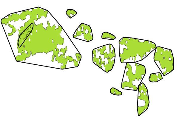
Fig. 9.11 Black lines identify the convex hull for each feature
Further reading: concave_hull, Convex hull algorithm
9.2.14.22. crosses
Tests whether a geometry crosses another. Returns TRUE if the supplied geometries have some, but not all, interior points in common.
Syntax |
crosses(geometry1, geometry2) |
Arguments |
|
Examples |
|
Further reading: overlay_crosses
9.2.14.23. densify_by_count
Takes a polygon or line layer geometry and generates a new one in which the geometries have a larger number of vertices than the original one.
Syntax |
densify_by_count(geometry, vertices) |
Arguments |
|
Examples |
|
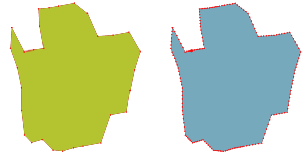
Fig. 9.12 Red points show the vertices before and after the densify
Further reading: Densify by count algorithm
9.2.14.24. densify_by_distance
Takes a polygon or line layer geometry and generates a new one in which the geometries are densified by adding additional vertices on edges that have a maximum distance of the specified interval distance.
Syntax |
densify_by_distance(geometry, distance) |
Arguments |
|
Examples |
|
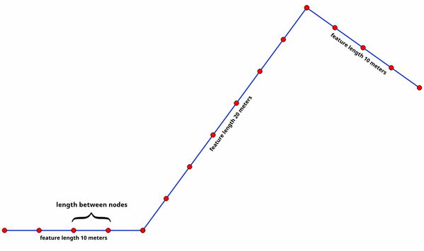
Fig. 9.13 Densify geometry at a given interval
Further reading: Densify by interval algorithm
9.2.14.25. difference
Returns a geometry that represents that part of geometry1 that does not intersect with geometry2.
Syntax |
difference(geometry1, geometry2) |
Arguments |
|
Examples |
|
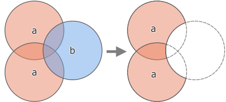
Fig. 9.14 Difference operation between a two-features input layer ‘a’ and a single feature overlay layer ‘b’ (left) - resulting in a new layer with the modified ‘a’ features (right)
Further reading: Difference algorithm
9.2.14.26. disjoint
Tests whether geometries do not spatially intersect. Returns TRUE if the geometries do not share any space together.
Syntax |
disjoint(geometry1, geometry2) |
Arguments |
|
Examples |
|
Further reading: overlay_disjoint
9.2.14.27. distance
Returns the minimum distance (based on spatial reference) between two geometries in projected units.
Syntax |
distance(geometry1, geometry2) |
Arguments |
|
Examples |
|
9.2.14.28. distance_to_vertex
Returns the distance along the geometry to a specified vertex.
Syntax |
distance_to_vertex(geometry, vertex) |
Arguments |
|
Examples |
|
9.2.14.29. end_point
Returns the last node from a geometry.
Syntax |
end_point(geometry) |
Arguments |
|
Examples |
|
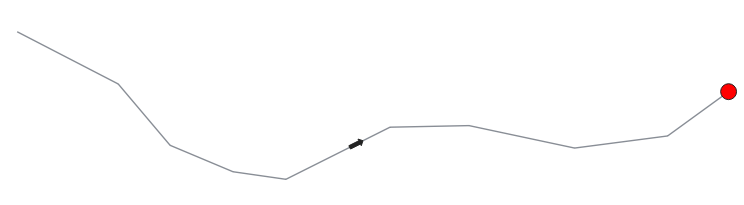
Fig. 9.15 End point of a line feature
Further reading: start_point, Extract specific vertices algorithm
9.2.14.30. equals
Alias for ‘equals_exact’ function with default geometry backend QGIS. Tests whether two geometries are point-by-point exactly equal. Note that the order of their vertices matters. Returns TRUE if geometry1 is exactly equal to geometry2.
Syntax |
equals(geometry1, geometry2) |
Arguments |
|
Examples |
|
Further reading: equals_exact, overlay_equals
9.2.14.31. equals_exact
Tests whether two geometries are point-by-point exactly equal. Note that the order of their vertices matters. Returns TRUE if geometry1 is exactly equal to geometry2.
Syntax |
equals_exact(geometry1, geometry2, [backend:=’QGIS’]) [] marks optional arguments |
Arguments |
|
Examples |
|
Further reading: equals, overlay_equals
9.2.14.32. equals_fuzzy
Tests whether two geometries are point-by-point equal in respect of a tolerance. Note that the order of their vertices matters. Returns TRUE if geometry1 is fuzzy equal to geometry2.
Syntax |
equals_fuzzy(geometry1, geometry2, [backend:=’QGIS’], [epsilon:=1e-8]) [] marks optional arguments |
Arguments |
|
Examples |
|
Further reading: overlay_equals_fuzzy, equals_exact
9.2.14.33. equals_topological
Tests whether two geometries are topologically equal. Returns TRUE if geometry1 is topologically equal to geometry2, i.e. opposite data direction and duplicated data are valid.
Syntax |
equals_topological(geometry1, geometry2, [backend:=’GEOS’]) [] marks optional arguments |
Arguments |
|
Examples |
|
Further reading: equals_exact, overlay_equals_topological
9.2.14.34. exif_geotag
Creates a point geometry from the exif geotags of an image file.
Syntax |
exif_geotag(path) |
Arguments |
|
Examples |
|
9.2.14.35. extend
Extends the start and end of a linestring geometry by a specified amount. Lines are extended using the bearing of the first and last segment in the line. For a multilinestring, all the parts are extended. Distances are in the Spatial Reference System of this geometry.
Syntax |
extend(geometry, start_distance, end_distance) |
Arguments |
|
Examples |
|
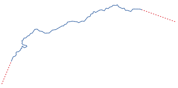
Fig. 9.16 The red dashes represent the initial and final extension of the original layer
Further reading: Extend lines algorithm
9.2.14.36. exterior_ring
Returns a line string representing the exterior ring of a polygon geometry. If the geometry is not a polygon then the result will be NULL.
Syntax |
exterior_ring(geometry) |
Arguments |
|
Examples |
|

Fig. 9.17 The dashed line represents the exterior ring of the polygon
Further reading: Boundary algorithm, interior_ring_n
9.2.14.37. extrude
Returns an extruded version of the input (Multi-)Curve or (Multi-)Linestring geometry with an extension specified by x and y.
Syntax |
extrude(geometry, x, y) |
Arguments |
|
Examples |
|
Fig. 9.18 Generating a polygon by extruding a line with offset in x and y directions
9.2.14.38. flip_coordinates
Returns a copy of the geometry with the x and y coordinates swapped. Useful for repairing geometries which have had their latitude and longitude values reversed.
Syntax |
flip_coordinates(geometry) |
Arguments |
|
Examples |
|
Further reading: Swap X and Y coordinates algorithm
9.2.14.39. force_polygon_ccw
Forces a geometry to respect the convention where exterior rings are counter-clockwise, interior rings are clockwise.
Syntax |
force_polygon_ccw(geometry) |
Arguments |
|
Examples |
|
Further reading: Force polygons counter-clockwise algorithm, force_polygon_cw, force_rhr
9.2.14.40. force_polygon_cw
Forces a geometry to respect the convention where exterior rings are clockwise, interior rings are counter-clockwise.
Syntax |
force_polygon_cw(geometry) |
Arguments |
|
Examples |
|
Further reading: Force polygons clockwise algorithm, force_polygon_ccw, force_rhr
9.2.14.41. force_rhr
Forces a geometry to respect the Right-Hand-Rule, in which the area that is bounded by a polygon is to the right of the boundary. In particular, the exterior ring is oriented in a clockwise direction and the interior rings in a counter-clockwise direction. Due to the inconsistency in the definition of the Right-Hand-Rule in some contexts it is recommended to use the explicit force_polygon_cw function instead.
Syntax |
force_rhr(geometry) |
Arguments |
|
Examples |
|
Further reading: Force right-hand-rule algorithm, force_polygon_ccw, force_polygon_cw
9.2.14.42. geom_from_gml
Returns a geometry from a GML representation of geometry.
Syntax |
geom_from_gml(gml) |
Arguments |
|
Examples |
|
9.2.14.43. geom_from_wkb
Returns a geometry created from a Well-Known Binary (WKB) representation.
Syntax |
geom_from_wkb(binary) |
Arguments |
|
Examples |
|
9.2.14.44. geom_from_wkt
Returns a geometry created from a Well-Known Text (WKT) representation.
Syntax |
geom_from_wkt(text) |
Arguments |
|
Examples |
|
9.2.14.45. geom_to_wkb
Returns the Well-Known Binary (WKB) representation of a geometry
Syntax |
geom_to_wkb(geometry) |
Arguments |
|
Examples |
|
9.2.14.46. geom_to_wkt
Returns the Well-Known Text (WKT) representation of the geometry without SRID metadata.
Syntax |
geom_to_wkt(geometry, [precision:=8]) [] marks optional arguments |
Arguments |
|
Examples |
|
9.2.14.47. $geometry
Returns the geometry of the current feature. Can be used for processing with other functions. WARNING: This function is deprecated. It is recommended to use the replacement @geometry variable instead.
Syntax |
$geometry |
Examples |
|
9.2.14.48. geometry
Returns a feature’s geometry.
Syntax |
geometry(feature) |
Arguments |
|
Examples |
|
9.2.14.49. geometry_n
Returns a specific geometry from a geometry collection, or NULL if the input geometry is not a collection. Also returns a part from a multipart geometry.
Syntax |
geometry_n(geometry, index) |
Arguments |
|
Examples |
|
9.2.14.50. geometry_type
Returns a string value describing the type of a geometry (Point, Line or Polygon)
Syntax |
geometry_type(geometry) |
Arguments |
|
Examples |
|
9.2.14.51. hausdorff_distance
Returns the Hausdorff distance between two geometries. This is basically a measure of how similar or dissimilar 2 geometries are, with a lower distance indicating more similar geometries.
The function can be executed with an optional densify fraction argument. If not specified, an approximation to the standard Hausdorff distance is used. This approximation is exact or close enough for a large subset of useful cases. Examples of these are:
computing distance between Linestrings that are roughly parallel to each other, and roughly equal in length. This occurs in matching linear networks.
Testing similarity of geometries.
If the default approximate provided by this method is insufficient, specify the optional densify fraction argument. Specifying this argument performs a segment densification before computing the discrete Hausdorff distance. The parameter sets the fraction by which to densify each segment. Each segment will be split into a number of equal-length subsegments, whose fraction of the total length is closest to the given fraction. Decreasing the densify fraction parameter will make the distance returned approach the true Hausdorff distance for the geometries.
Syntax |
hausdorff_distance(geometry1, geometry2, [densify_fraction:=1]) [] marks optional arguments |
Arguments |
|
Examples |
|
9.2.14.52. inclination
Returns the inclination measured from the zenith (0) to the nadir (180) on point1 to point2.
Syntax |
inclination(point1, point2) |
Arguments |
|
Examples |
|
9.2.14.53. interior_ring_n
Returns a specific interior ring from a polygon geometry, or NULL if the geometry is not a polygon.
Syntax |
interior_ring_n(geometry, index) |
Arguments |
|
Examples |
|

Fig. 9.19 The dashed line represents a specific interior ring of the polygon
Further reading: exterior_ring
9.2.14.54. intersection
Returns a geometry that represents the shared portion of two geometries.
Syntax |
intersection(geometry1, geometry2) |
Arguments |
|
Examples |
|
Further reading: Intersection algorithm
9.2.14.55. intersects
Tests whether a geometry intersects another. Returns TRUE if the geometries spatially intersect (share any portion of space) and false if they do not.
Syntax |
intersects(geometry1, geometry2) |
Arguments |
|
Examples |
|
Further reading: overlay_intersects
9.2.14.56. intersects_bbox
Tests whether a geometry’s bounding box overlaps another geometry’s bounding box. Returns TRUE if the geometries spatially intersect the bounding box defined and false if they do not.
Syntax |
intersects_bbox(geometry1, geometry2) |
Arguments |
|
Examples |
|
9.2.14.57. is_closed
Returns TRUE if a line string is closed (start and end points are coincident), or false if a line string is not closed. If the geometry is not a line string then the result will be NULL.
Syntax |
is_closed(geometry) |
Arguments |
|
Examples |
|
9.2.14.58. is_empty
Returns TRUE if a geometry is empty (without coordinates), false if the geometry is not empty and NULL if there is no geometry. See also is_empty_or_null.
Syntax |
is_empty(geometry) |
Arguments |
|
Examples |
|
Further reading: is_empty_or_null
9.2.14.59. is_empty_or_null
Returns TRUE if a geometry is NULL or empty (without coordinates) or false otherwise. This function is like the expression ‘@geometry IS NULL or is_empty(@geometry)’
Syntax |
is_empty_or_null(geometry) |
Arguments |
|
Examples |
|
9.2.14.60. is_multipart
Returns TRUE if the geometry is of Multi type.
Syntax |
is_multipart(geometry) |
Arguments |
|
Examples |
|
9.2.14.61. is_valid
Returns TRUE if a geometry is valid; if it is well-formed in 2D according to the OGC rules.
Syntax |
is_valid(geometry) |
Arguments |
|
Examples |
|
Further reading: make_valid, Check validity algorithm
9.2.14.62. $length
Returns the length of a linestring. If you need the length of a border of a polygon, use $perimeter instead. The length calculated by this function respects both the current project’s ellipsoid setting and distance unit settings. For example, if an ellipsoid has been set for the project then the calculated length will be ellipsoidal, and if no ellipsoid is set then the calculated length will be planimetric.
Syntax |
$length |
Examples |
|
9.2.14.63. length
Returns the number of characters in a string or the length of a geometry linestring.
String variant
Returns the number of characters in a string.
Syntax |
length(string) |
Arguments |
|
Examples |
|
Geometry variant
Calculate the length of a geometry line object. Calculations are always planimetric in the Spatial Reference System (SRS) of this geometry, and the units of the returned length will match the units for the SRS. This differs from the calculations performed by the $length function, which will perform ellipsoidal calculations based on the project’s ellipsoid and distance unit settings.
Syntax |
length(geometry) |
Arguments |
|
Examples |
|
Further reading: straight_distance_2d
9.2.14.64. length3D
Calculates the 3D length of a geometry line object. If the geometry is not a 3D line object, it returns its 2D length. Calculations are always planimetric in the Spatial Reference System (SRS) of this geometry, and the units of the returned length will match the units for the SRS. This differs from the calculations performed by the $length function, which will perform ellipsoidal calculations based on the project’s ellipsoid and distance unit settings.
Syntax |
length3D(geometry) |
Arguments |
|
Examples |
|
9.2.14.65. line_interpolate_angle
Returns the angle parallel to the geometry at a specified distance along a linestring geometry. Angles are in degrees clockwise from north.
Syntax |
line_interpolate_angle(geometry, distance) |
Arguments |
|
Examples |
|
9.2.14.66. line_interpolate_point
Returns the point interpolated by a specified distance along a linestring geometry.
Syntax |
line_interpolate_point(geometry, distance) |
Arguments |
|
Examples |
|
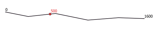
Fig. 9.20 Interpolated point at 500m of the beginning of the line
Further reading: Interpolate point on line algorithm
9.2.14.67. line_interpolate_point_by_m
Returns the point interpolated by a matching M value along a linestring geometry.
Syntax |
line_interpolate_point_by_m(geometry, m, [use_3d_distance:=false]) [] marks optional arguments |
Arguments |
|
Examples |
|
9.2.14.68. line_locate_m
Returns the distance along a linestring corresponding to the first matching interpolated M value.
Syntax |
line_locate_m(geometry, m, [use_3d_distance:=false]) [] marks optional arguments |
Arguments |
|
Examples |
|
9.2.14.69. line_locate_point
Returns the distance along a linestring corresponding to the closest position the linestring comes to a specified point geometry.
Syntax |
line_locate_point(geometry, point) |
Arguments |
|
Examples |
|
9.2.14.70. line_merge
Returns a LineString or MultiLineString geometry, where any connected LineStrings from the input geometry have been merged into a single linestring. This function will return NULL if passed a geometry which is not a LineString/MultiLineString.
Syntax |
line_merge(geometry) |
Arguments |
|
Examples |
|
9.2.14.71. line_substring
Returns the portion of a line (or curve) geometry which falls between the specified start and end distances (measured from the beginning of the line). Z and M values are linearly interpolated from existing values.
Syntax |
line_substring(geometry, start_distance, end_distance) |
Arguments |
|
Examples |
|
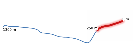
Fig. 9.21 Substring line with starting distance set at 0 meters and the ending distance at 250 meters.
Further reading: Line substring algorithm
9.2.14.72. m
Returns the m (measure) value of a point geometry.
Syntax |
m(geometry) |
Arguments |
|
Examples |
|
9.2.14.73. m_at
Retrieves a m coordinate of the geometry, or NULL if the geometry has no m value.
Syntax |
m_at(geometry, vertex) |
Arguments |
|
Examples |
|
9.2.14.74. m_max
Returns the maximum m (measure) value of a geometry.
Syntax |
m_max(geometry) |
Arguments |
|
Examples |
|
9.2.14.75. m_min
Returns the minimum m (measure) value of a geometry.
Syntax |
m_min(geometry) |
Arguments |
|
Examples |
|
9.2.14.76. main_angle
Returns the angle of the long axis (clockwise, in degrees from North) of the oriented minimal bounding rectangle, which completely covers the geometry.
Syntax |
main_angle(geometry) |
Arguments |
|
Examples |
|
9.2.14.77. make_circle
Creates a circular polygon.
Syntax |
make_circle(center, radius, [segments:=36]) [] marks optional arguments |
Arguments |
|
Examples |
|
9.2.14.78. make_ellipse
Creates an elliptical polygon.
Syntax |
make_ellipse(center, semi_major_axis, semi_minor_axis, azimuth, [segments:=36]) [] marks optional arguments |
Arguments |
|
Examples |
|
9.2.14.79. make_line
Creates a line geometry from a series of point geometries.
List of arguments variant
Line vertices are specified as separate arguments to the function.
Syntax |
make_line(point1, point2, …) |
Arguments |
|
Examples |
|
Array variant
Line vertices are specified as an array of points.
Syntax |
make_line(array) |
Arguments |
|
Examples |
|
9.2.14.80. make_point
Creates a point geometry from an x and y (and optional z and m) value.
Syntax |
make_point(x, y, [z], [m]) [] marks optional arguments |
Arguments |
|
Examples |
|
9.2.14.81. make_point_m
Creates a point geometry from an x, y coordinate and m value.
Syntax |
make_point_m(x, y, m) |
Arguments |
|
Examples |
|
9.2.14.82. make_polygon
Creates a polygon geometry from an outer ring and optional series of inner ring geometries.
Syntax |
make_polygon(outerRing, [innerRing1], [innerRing2], …) [] marks optional arguments |
Arguments |
|
Examples |
|
9.2.14.83. make_rectangle_3points
Creates a rectangle from 3 points, the first two of which define its first side.
Syntax |
make_rectangle_3points(point1, point2, point3, [option:=0]) [] marks optional arguments |
Arguments |
|
Examples |
|
9.2.14.84. make_regular_polygon
Creates a regular polygon.
Syntax |
make_regular_polygon(center, radius, number_sides, [circle:=0]) [] marks optional arguments |
Arguments |
|
Examples |
|
9.2.14.85. make_square
Creates a square from a diagonal.
Syntax |
make_square(point1, point2) |
Arguments |
|
Examples |
|
9.2.14.86. make_triangle
Creates a triangle polygon.
Syntax |
make_triangle(point1, point2, point3) |
Arguments |
|
Examples |
|
9.2.14.87. make_valid
Returns a valid geometry or an empty geometry if the geometry could not be made valid.
Syntax |
make_valid(geometry, [method:=’structure’], [keep_collapsed:=false]) [] marks optional arguments |
Arguments |
|
Examples |
|
Further reading: is_valid, Fix geometries algorithm
9.2.14.88. minimal_circle
Returns the minimal enclosing circle of a geometry. It represents the minimum circle that encloses all geometries within the set.
Syntax |
minimal_circle(geometry, [segments:=36]) [] marks optional arguments |
Arguments |
|
Examples |
|
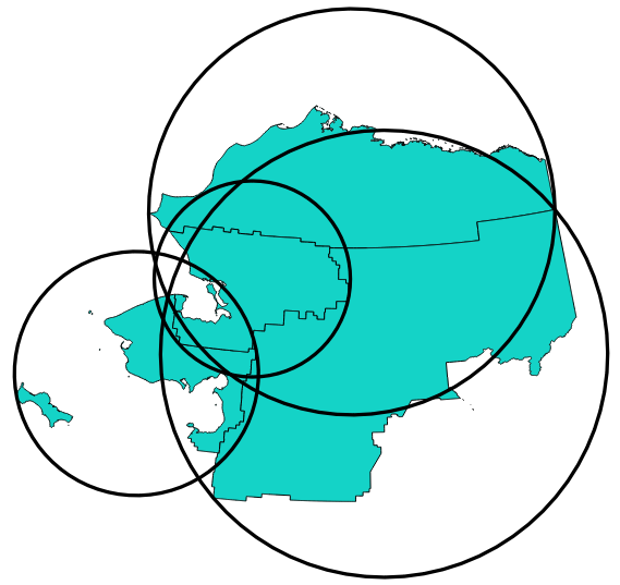
Fig. 9.22 Minimal enclosing circle of each feature
Further reading: Minimum enclosing circles algorithm
9.2.14.89. nodes_to_points
Returns a multipoint geometry consisting of every node in the input geometry.
Syntax |
nodes_to_points(geometry, [ignore_closing_nodes:=false]) [] marks optional arguments |
Arguments |
|
Examples |
|
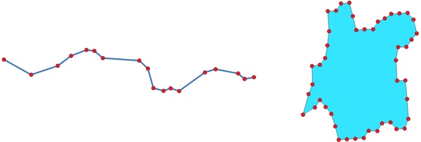
Fig. 9.23 Multi-point feature extracted from vertices
Further reading: Extract vertices algorithm
9.2.14.90. num_geometries
Returns the number of geometries in a geometry collection, or the number of parts in a multi-part geometry. The function returns NULL if the input geometry is not a collection.
Syntax |
num_geometries(geometry) |
Arguments |
|
Examples |
|
9.2.14.91. num_interior_rings
Returns the number of interior rings in a polygon or geometry collection, or NULL if the input geometry is not a polygon or collection.
Syntax |
num_interior_rings(geometry) |
Arguments |
|
Examples |
|
9.2.14.92. num_points
Returns the number of vertices in a geometry.
Syntax |
num_points(geometry) |
Arguments |
|
Examples |
|
9.2.14.93. num_rings
Returns the number of rings (including exterior rings) in a polygon or geometry collection, or NULL if the input geometry is not a polygon or collection.
Syntax |
num_rings(geometry) |
Arguments |
|
Examples |
|
9.2.14.94. offset_curve
Returns a geometry formed by offsetting a linestring geometry to the side. Distances are in the Spatial Reference System of this geometry.
Syntax |
offset_curve(geometry, distance, [segments:=8], [join:=1], [miter_limit:=2.0]) [] marks optional arguments |
Arguments |
|
Examples |
|
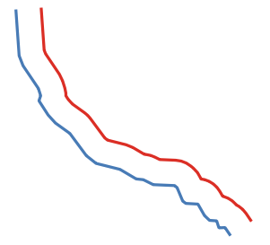
Fig. 9.24 In blue the source layer, in red the offset one
Further reading: Offset lines algorithm
9.2.14.95. order_parts
Orders the parts of a MultiGeometry by a given criteria
Syntax |
order_parts(geometry, orderby, [ascending:=true]) [] marks optional arguments |
Arguments |
|
Examples |
|
9.2.14.96. oriented_bbox
Returns a geometry which represents the minimal oriented bounding box of an input geometry.
Syntax |
oriented_bbox(geometry) |
Arguments |
|
Examples |
|
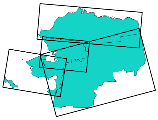
Fig. 9.25 Oriented minimum bounding box
Further reading: Oriented minimum bounding box algorithm
9.2.14.97. overlaps
Tests whether a geometry overlaps another. Returns TRUE if the geometries share space, are of the same dimension, but are not completely contained by each other.
Syntax |
overlaps(geometry1, geometry2) |
Arguments |
|
Examples |
|
9.2.14.98. overlay_contains
Returns whether the current feature spatially contains at least one feature from a target layer, or returns an array of expression-based results for the features in the target layer contained in the current feature.
Read more on the underlying GEOS “Contains” predicate, as described in PostGIS ST_Contains function.
Syntax |
overlay_contains(layer, [expression], [filter], [limit], [cache:=false]) [] marks optional arguments |
Arguments |
|
Examples |
|
Further reading: contains, array manipulation, Select by location algorithm
9.2.14.99. overlay_crosses
Returns whether the current feature spatially crosses at least one feature from a target layer, or returns an array of expression-based results for the features in the target layer crossed by the current feature.
Read more on the underlying GEOS “Crosses” predicate, as described in PostGIS ST_Crosses function.
Syntax |
overlay_crosses(layer, [expression], [filter], [limit], [cache:=false]) [] marks optional arguments |
Arguments |
|
Examples |
|
Further reading: crosses, array manipulation, Select by location algorithm
9.2.14.100. overlay_disjoint
Returns whether the current feature is spatially disjoint from all the features of a target layer, or returns an array of expression-based results for the features in the target layer that are disjoint from the current feature.
Read more on the underlying GEOS “Disjoint” predicate, as described in PostGIS ST_Disjoint function.
Syntax |
overlay_disjoint(layer, [expression], [filter], [limit], [cache:=false]) [] marks optional arguments |
Arguments |
|
Examples |
|
Further reading: disjoint, array manipulation, Select by location algorithm
9.2.14.101. overlay_equals
Alias for ‘overlay_equals_exact’ function with default geometry backend QGIS. Returns whether the current feature’s geometry is exactly equal to at least one feature’s geometry from a target layer, or returns an array of expression-based results for the features in the target layer whose geometry is exactly equal to the current feature’s geometry. Note that the order of vertices matters.
Syntax |
overlay_equals(layer, [expression], [filter], [limit], [cache:=false]) [] marks optional arguments |
Arguments |
|
Examples |
|
Note
This function requires exact equality of geometries, meaning that the geometries ‘LINESTRING( 0 0, 1 1 )’ and ‘LINESTRING( 1 1, 0 0 )’ are different.
Further reading: overlay_equals_exact, equals, array manipulation
9.2.14.102. overlay_equals_exact
Returns whether the current feature’s geometry is point-by-point exactly equal to at least one feature’s geometry from a target layer, or returns an array of expression-based results for the features in the target layer whose geometry is exactly equal to the current feature’s geometry. Note that the order of vertices matters.
Syntax |
overlay_equals_exact(layer, [expression], [filter], [limit], [cache:=false], [backend:=’QGIS’]) [] marks optional arguments |
Arguments |
|
Examples |
|
Note
This function requires exact equality of geometries, meaning that the geometries ‘LINESTRING( 0 0, 1 1 )’ and ‘LINESTRING( 1 1, 0 0 )’ are different.
Further reading: overlay_equals, equals_exact, array manipulation
9.2.14.103. overlay_equals_fuzzy
Returns whether the current feature’s geometry is point-by-point equal in respect of a tolerance to at least one feature’s geometry from a target layer, or returns an array of expression-based results for the features in the target layer whose geometry is fuzzy equal to the current feature’s geometry. Note that the order of vertices matters.
Syntax |
overlay_equals_fuzzy(layer, [expression], [filter], [limit], [cache:=false], [backend:=’QGIS’], [epsilon:=1e-8]) [] marks optional arguments |
Arguments |
|
Examples |
|
Note
This function uses fuzzy equality of geometries, see also ‘equals_fuzzy’ function examples.
Further reading: equals_fuzzy, overlay_equals_exact, array manipulation
9.2.14.104. overlay_equals_topological
Returns whether the current feature’s geometry is topologically equal to at least one feature’s geometry from a target layer, or returns an array of expression-based results for the features in the target layer whose geometry is topologically equal to the current feature’s geometry. See also ‘equals_topological’ function.
Syntax |
overlay_equals_topological(layer, [expression], [filter], [limit], [cache:=false], [backend:=’GEOS’]) [] marks optional arguments |
Arguments |
|
Examples |
|
Note
This function uses topological equality of geometries, see also ‘equals_topological’ function examples.
Further reading: overlay_equals_exact, equals_topological, array manipulation,
9.2.14.105. overlay_intersects
Returns whether the current feature spatially intersects at least one feature from a target layer, or returns an array of expression-based results for the features in the target layer intersected by the current feature.
Read more on the underlying GEOS “Intersects” predicate, as described in PostGIS ST_Intersects function.
Syntax |
overlay_intersects(layer, [expression], [filter], [limit], [cache:=false], [min_overlap], [min_inscribed_circle_radius], [return_details], [sort_by_intersection_size]) [] marks optional arguments |
Arguments |
|
Examples |
|
Further reading: intersects, array manipulation, Select by location algorithm
9.2.14.106. overlay_nearest
Returns whether the current feature has feature(s) from a target layer within a given distance, or returns an array of expression-based results for the features in the target layer within a distance from the current feature.
Note: This function can be slow and consume a lot of memory for large layers.
Syntax |
overlay_nearest(layer, [expression], [filter], [limit:=1], [max_distance], [cache:=false]) [] marks optional arguments |
Arguments |
|
Examples |
|
Further reading: array manipulation, Join attributes by nearest algorithm
9.2.14.107. overlay_touches
Returns whether the current feature spatially touches at least one feature from a target layer, or returns an array of expression-based results for the features in the target layer touched by the current feature.
Read more on the underlying GEOS “Touches” predicate, as described in PostGIS ST_Touches function.
Syntax |
overlay_touches(layer, [expression], [filter], [limit], [cache:=false]) [] marks optional arguments |
Arguments |
|
Examples |
|
Further reading: touches, array manipulation, Select by location algorithm
9.2.14.108. overlay_within
Returns whether the current feature is spatially within at least one feature from a target layer, or an array of expression-based results for the features in the target layer that contain the current feature.
Read more on the underlying GEOS “Within” predicate, as described in PostGIS ST_Within function.
Syntax |
overlay_within(layer, [expression], [filter], [limit], [cache:=false]) [] marks optional arguments |
Arguments |
|
Examples |
|
Further reading: within, array manipulation, Select by location algorithm
9.2.14.109. $perimeter
Returns the perimeter length of the current feature. The perimeter calculated by this function respects both the current project’s ellipsoid setting and distance unit settings. For example, if an ellipsoid has been set for the project then the calculated perimeter will be ellipsoidal, and if no ellipsoid is set then the calculated perimeter will be planimetric.
Syntax |
$perimeter |
Examples |
|
9.2.14.110. perimeter
Returns the perimeter of a geometry polygon object. Calculations are always planimetric in the Spatial Reference System (SRS) of this geometry, and the units of the returned perimeter will match the units for the SRS. This differs from the calculations performed by the $perimeter function, which will perform ellipsoidal calculations based on the project’s ellipsoid and distance unit settings.
Syntax |
perimeter(geometry) |
Arguments |
|
Examples |
|
9.2.14.111. point_n
Returns a specific node from a geometry.
Syntax |
point_n(geometry, index) |
Arguments |
|
Examples |
|
Further reading: Extract specific vertices algorithm
9.2.14.112. point_on_surface
Returns a point guaranteed to lie on the surface of a geometry.
Syntax |
point_on_surface(geometry) |
Arguments |
|
Examples |
|
Further reading: Point on Surface algorithm
9.2.14.113. pole_of_inaccessibility
Calculates the approximate pole of inaccessibility for a surface, which is the most distant internal point from the boundary of the surface. This function uses the ‘polylabel’ algorithm (Vladimir Agafonkin, 2016), which is an iterative approach guaranteed to find the true pole of inaccessibility within a specified tolerance. More precise tolerances require more iterations and will take longer to calculate.
Syntax |
pole_of_inaccessibility(geometry, tolerance) |
Arguments |
|
Examples |
|
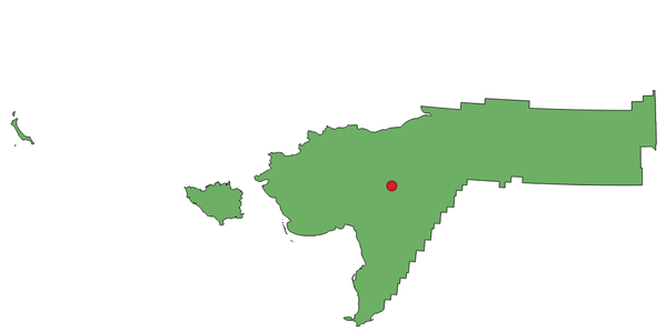
Fig. 9.26 Pole of inaccessibility
Further reading: Pole of inaccessibility algorithm
9.2.14.114. project
Returns a point projected from a start point using a distance, a bearing (azimuth) and an elevation in radians.
Syntax |
project(point, distance, azimuth, [elevation]) [] marks optional arguments |
Arguments |
|
Examples |
|
Further reading: Project points (Cartesian) algorithm
9.2.14.115. relate
Tests the Dimensional Extended 9 Intersection Model (DE-9IM) representation of the relationship between two geometries.
Relationship variant
Returns the Dimensional Extended 9 Intersection Model (DE-9IM) representation of the relationship between two geometries.
Syntax |
relate(geometry1, geometry2) |
Arguments |
|
Examples |
|
Pattern match variant
Tests whether the DE-9IM relationship between two geometries matches a specified pattern.
Syntax |
relate(geometry1, geometry2, pattern) |
Arguments |
|
Examples |
|
9.2.14.116. reverse
Reverses the direction of a line string or reverses a string of text.
String variant
Reverses the order of characters in a string.
Syntax |
reverse(string) |
Arguments |
|
Examples |
|
Geometry variant
Reverses the direction of a line string by reversing the order of its vertices.
Syntax |
reverse(geometry) |
Arguments |
|
Examples |
|
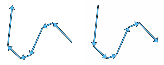
Fig. 9.27 Reversing line direction
Further reading: Reverse line direction algorithm
9.2.14.117. rotate
Returns a rotated version of a geometry. Calculations are in the Spatial Reference System of this geometry.
Syntax |
rotate(geometry, rotation, [center:=NULL], [per_part:=false]) [] marks optional arguments |
Arguments |
|
Examples |
|
Fig. 9.28 Rotating features
9.2.14.118. roundness
Calculates how close a polygon shape is to a circle. The function returns 1 when the polygon shape is a perfect circle and 0 when it is completely flat.
Syntax |
roundness(geometry) |
Arguments |
|
Examples |
|
Further reading: Roundness algorithm
9.2.14.119. scale
Returns a scaled version of a geometry. Calculations are in the Spatial Reference System of this geometry.
Syntax |
scale(geometry, x_scale, y_scale, [center:=NULL]) [] marks optional arguments |
Arguments |
|
Examples |
|
9.2.14.120. segments_to_lines
Returns a multi line geometry consisting of a line for every segment in the input geometry.
Syntax |
segments_to_lines(geometry) |
Arguments |
|
Examples |
|
Further reading: Explode lines algorithm
9.2.14.122. shortest_line
Returns the shortest line joining geometry1 to geometry2. The resultant line will start at geometry1 and end at geometry2.
Syntax |
shortest_line(geometry1, geometry2) |
Arguments |
|
Examples |
|
9.2.14.123. simplify
Simplifies a geometry by removing nodes using a distance based threshold (ie, the Douglas Peucker algorithm). The algorithm preserves large deviations in geometries and reduces the number of vertices in nearly straight segments.
Syntax |
simplify(geometry, tolerance) |
Arguments |
|
Examples |
|
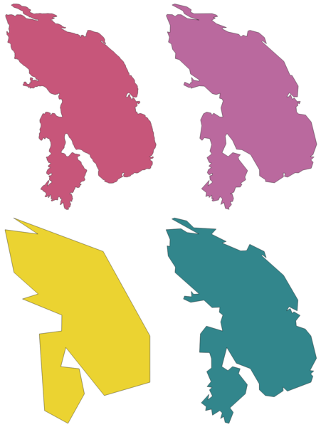
Fig. 9.29 From left to right, source layer and increasing simplification tolerances
Further reading: Simplify algorithm
9.2.14.124. simplify_vw
Simplifies a geometry by removing nodes using an area based threshold (ie, the Visvalingam-Whyatt algorithm). The algorithm removes vertices which create small areas in geometries, e.g., narrow spikes or nearly straight segments.
Syntax |
simplify_vw(geometry, tolerance) |
Arguments |
|
Examples |
|
Further reading: Simplify algorithm
9.2.14.125. single_sided_buffer
Returns a geometry formed by buffering out just one side of a linestring geometry. Distances are in the Spatial Reference System of this geometry.
Syntax |
single_sided_buffer(geometry, distance, [segments:=8], [join:=1], [miter_limit:=2.0]) [] marks optional arguments |
Arguments |
|
Examples |
|
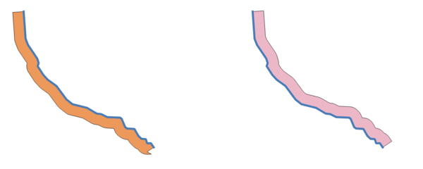
Fig. 9.30 Left versus right side buffer on the same vector line layer
Further reading: Single sided buffer algorithm
9.2.14.126. sinuosity
Returns the sinuosity of a curve, which is the ratio of the curve length to the straight (2D) distance between its endpoints.
Syntax |
sinuosity(geometry) |
Arguments |
|
Examples |
|
9.2.14.127. smooth
Smooths a geometry by adding extra nodes which round off corners in the geometry. If input geometries contain Z or M values, these will also be smoothed and the output geometry will retain the same dimensionality as the input geometry.
Syntax |
smooth(geometry, [iterations:=1], [offset:=0.25], [min_length:=-1], [max_angle:=180]) [] marks optional arguments |
Arguments |
|
Examples |
|
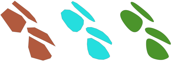
Fig. 9.31 Increasing number of iterations causes smoother geometries
Further reading: Smooth algorithm
9.2.14.128. square_wave
Constructs square/rectangular waves along the boundary of a geometry.
Syntax |
square_wave(geometry, wavelength, amplitude, [strict:=false]) [] marks optional arguments |
Arguments |
|
Examples |
|
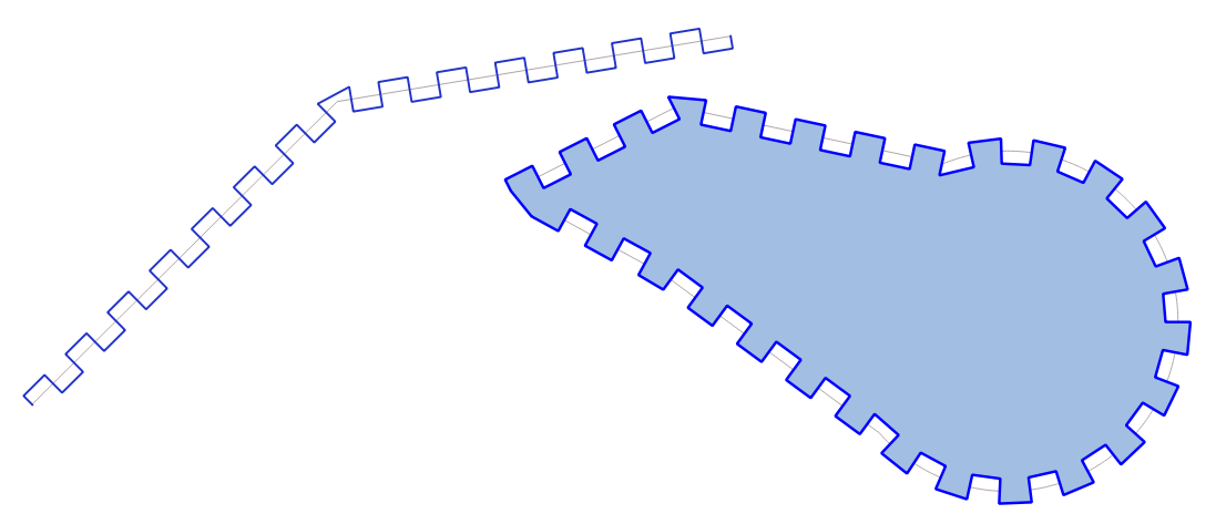
Fig. 9.32 Symbolizing features with square waves
9.2.14.129. square_wave_randomized
Constructs randomized square/rectangular waves along the boundary of a geometry.
Syntax |
square_wave_randomized(geometry, min_wavelength, max_wavelength, min_amplitude, max_amplitude, [seed:=0]) [] marks optional arguments |
Arguments |
|
Examples |
|
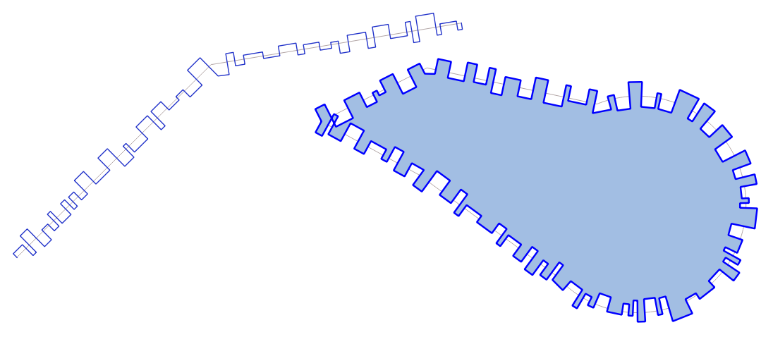
Fig. 9.33 Symbolizing features with square randomized waves
9.2.14.130. start_point
Returns the first node from a geometry.
Syntax |
start_point(geometry) |
Arguments |
|
Examples |
|
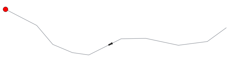
Fig. 9.34 Starting point of a line feature
Further reading: end_point, Extract specific vertices algorithm
9.2.14.131. straight_distance_2d
Returns the direct/euclidean distance between the first and last vertex of a geometry. The geometry must be a curve (circularstring, linestring).
Syntax |
straight_distance_2d(geometry) |
Arguments |
|
Examples |
|
Further reading: length
9.2.14.132. sym_difference
Returns a geometry that represents the portions of two geometries that do not intersect.
Syntax |
sym_difference(geometry1, geometry2) |
Arguments |
|
Examples |
|
Further reading: Symmetrical difference algorithm
9.2.14.133. tapered_buffer
Creates a buffer along a line geometry where the buffer diameter varies evenly over the length of the line.
Syntax |
tapered_buffer(geometry, start_width, end_width, [segments:=8]) [] marks optional arguments |
Arguments |
|
Examples |
|
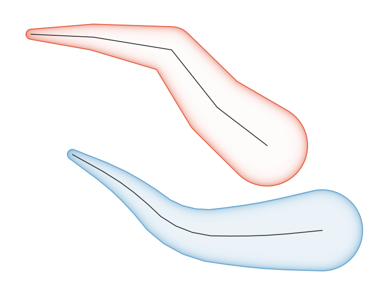
Fig. 9.35 Tapered buffer on line features
Further reading: Tapered buffers algorithm
9.2.14.134. touches
Tests whether a geometry touches another. Returns TRUE if the geometries have at least one point in common, but their interiors do not intersect.
Syntax |
touches(geometry1, geometry2) |
Arguments |
|
Examples |
|
Further reading: overlay_touches
9.2.14.135. transform
Returns the geometry transformed from a source CRS to a destination CRS.
Syntax |
transform(geometry, source_auth_id, dest_auth_id) |
Arguments |
|
Examples |
|
Further reading: Reproject layer algorithm
9.2.14.136. translate
Returns a translated version of a geometry. Calculations are in the Spatial Reference System of this geometry.
Syntax |
translate(geometry, dx, dy) |
Arguments |
|
Examples |
|
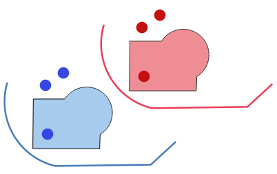
Fig. 9.36 Translating features
Further reading: Translate algorithm
9.2.14.137. triangular_wave
Constructs triangular waves along the boundary of a geometry.
Syntax |
triangular_wave(geometry, wavelength, amplitude, [strict:=false]) [] marks optional arguments |
Arguments |
|
Examples |
|
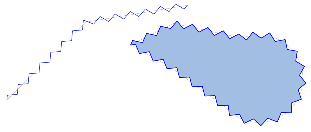
Fig. 9.37 Symbolizing features with triangular waves
9.2.14.138. triangular_wave_randomized
Constructs randomized triangular waves along the boundary of a geometry.
Syntax |
triangular_wave_randomized(geometry, min_wavelength, max_wavelength, min_amplitude, max_amplitude, [seed:=0]) [] marks optional arguments |
Arguments |
|
Examples |
|
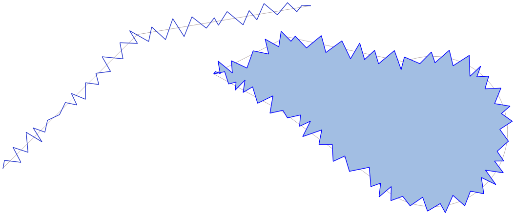
Fig. 9.38 Symbolizing features with triangular randomized waves
9.2.14.139. union
Returns a geometry that represents the point set union of the geometries.
Syntax |
union(geometry1, geometry2) |
Arguments |
|
Examples |
|
9.2.14.140. wave
Constructs rounded (sine-like) waves along the boundary of a geometry.
Syntax |
wave(geometry, wavelength, amplitude, [strict:=false]) [] marks optional arguments |
Arguments |
|
Examples |
|
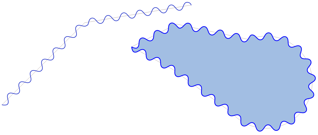
Fig. 9.39 Symbolizing features with waves
9.2.14.141. wave_randomized
Constructs randomized curved (sine-like) waves along the boundary of a geometry.
Syntax |
wave_randomized(geometry, min_wavelength, max_wavelength, min_amplitude, max_amplitude, [seed:=0]) [] marks optional arguments |
Arguments |
|
Examples |
|
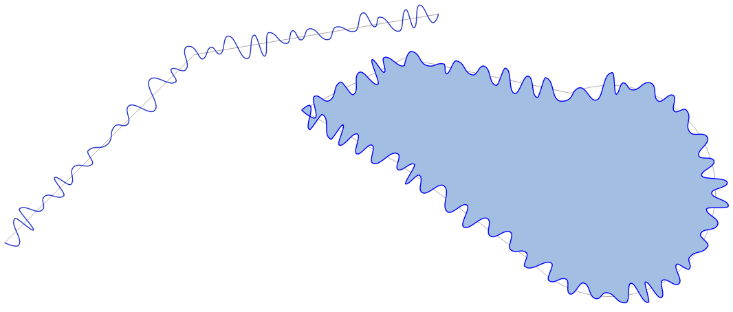
Fig. 9.40 Symbolizing features with randomized waves
9.2.14.142. wedge_buffer
Returns a wedge shaped buffer originating from a point geometry.
Syntax |
wedge_buffer(center, azimuth, width, outer_radius, [inner_radius:=0.0]) [] marks optional arguments |
Arguments |
|
Examples |
|
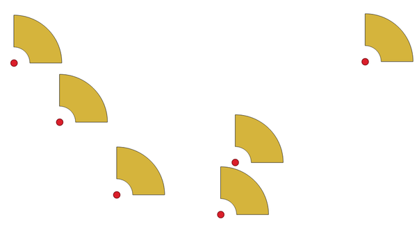
Fig. 9.41 Wedge buffering features
Further reading: Create wedge buffers algorithm
9.2.14.143. within
Tests whether a geometry is within another. Returns TRUE if the geometry1 is completely within geometry2.
Syntax |
within(geometry1, geometry2) |
Arguments |
|
Examples |
|
Further reading: overlay_within
9.2.14.144. $x
Returns the x coordinate of the current point feature. If the feature is a multipoint feature, then the x-coordinate of the first point will be returned. WARNING: This function is deprecated. It is recommended to use the replacement x() function with @geometry variable instead.
Syntax |
$x |
Examples |
|
Further reading: x
9.2.14.145. x
Returns the x coordinate of a point geometry, or the x coordinate of the centroid for a non-point geometry.
Syntax |
x(geometry) |
Arguments |
|
Examples |
|
9.2.14.146. $x_at
Retrieves a x coordinate of the current feature’s geometry. WARNING: This function is deprecated. It is recommended to use the replacement x_at function with @geometry variable instead.
Syntax |
$x_at(vertex) |
Arguments |
|
Examples |
|
Further reading: x_at
9.2.14.147. x_at
Retrieves a x coordinate of the geometry.
Syntax |
x_at(geometry, vertex) |
Arguments |
|
Examples |
|
9.2.14.148. x_max
Returns the maximum x coordinate of a geometry. Calculations are in the spatial reference system of this geometry.
Syntax |
x_max(geometry) |
Arguments |
|
Examples |
|
9.2.14.149. x_min
Returns the minimum x coordinate of a geometry. Calculations are in the spatial reference system of this geometry.
Syntax |
x_min(geometry) |
Arguments |
|
Examples |
|
9.2.14.150. $y
Returns the y coordinate of the current point feature. If the feature is a multipoint feature, then the y-coordinate of the first point will be returned. WARNING: This function is deprecated. It is recommended to use the replacement y() function with @geometry variable instead.
Syntax |
$y |
Examples |
|
Further reading: y
9.2.14.151. y
Returns the y coordinate of a point geometry, or the y coordinate of the centroid for a non-point geometry.
Syntax |
y(geometry) |
Arguments |
|
Examples |
|
9.2.14.152. $y_at
Retrieves a y coordinate of the current feature’s geometry. WARNING: This function is deprecated. It is recommended to use the replacement y_at function with @geometry variable instead.
Syntax |
$y_at(vertex) |
Arguments |
|
Examples |
|
Further reading: y_at
9.2.14.153. y_at
Retrieves a y coordinate of the geometry.
Syntax |
y_at(geometry, vertex) |
Arguments |
|
Examples |
|
9.2.14.154. y_max
Returns the maximum y coordinate of a geometry. Calculations are in the spatial reference system of this geometry.
Syntax |
y_max(geometry) |
Arguments |
|
Examples |
|
9.2.14.155. y_min
Returns the minimum y coordinate of a geometry. Calculations are in the spatial reference system of this geometry.
Syntax |
y_min(geometry) |
Arguments |
|
Examples |
|
9.2.14.156. $z
Returns the z value of the current point feature if it is 3D. If the feature is a multipoint feature, then the z value of the first point will be returned. WARNING: This function is deprecated. It is recommended to use the replacement z() function with @geometry variable instead.
Syntax |
$z |
Examples |
|
9.2.14.157. z
Returns the z coordinate of a point geometry, or NULL if the geometry has no z value.
Syntax |
z(geometry) |
Arguments |
|
Examples |
|
9.2.14.158. z_at
Retrieves a z coordinate of the geometry, or NULL if the geometry has no z value.
Syntax |
z_at(geometry, vertex) |
Arguments |
|
Examples |
|
9.2.14.159. z_max
Returns the maximum z coordinate of a geometry, or NULL if the geometry has no z value.
Syntax |
z_max(geometry) |
Arguments |
|
Examples |
|
9.2.14.160. z_min
Returns the minimum z coordinate of a geometry, or NULL if the geometry has no z value.
Syntax |
z_min(geometry) |
Arguments |
|
Examples |
|
9.2.15. Layout Functions
This group contains functions to manipulate print layout items properties.
Show/hide list of functions
9.2.15.1. item_variables
Returns a map of variables from a layout item inside this print layout.
Syntax |
item_variables(id) |
Arguments |
|
Examples |
|
Further reading: List of default variables
9.2.15.2. map_credits
Returns a list of credit (usage rights) strings for the layers shown in a layout, or specific layout map item.
Syntax |
map_credits([id], [include_layer_names:=false], [layer_name_separator:=’: ‘]) [] marks optional arguments |
Arguments |
|
Examples |
|
This function requires the Access metadata properties of the layers to have been filled.
9.2.16. Magnetic Models Functions
This group contains functions that calculate values based on magnetic models.
Show/hide list of functions
9.2.16.1. magnetic_declination
Returns the declination of a magnetic field at a point, in degrees east of north
Syntax |
magnetic_declination(model_name, date, latitude, longitude, height, [model_path]) [] marks optional arguments |
Arguments |
|
Examples |
|
9.2.16.2. magnetic_declination_rate_of_change
Returns the rate of change of the declination of a magnetic field at a point, in degrees per year
Syntax |
magnetic_declination_rate_of_change(model_name, date, latitude, longitude, height, [model_path]) [] marks optional arguments |
Arguments |
|
Examples |
|
9.2.16.3. magnetic_inclination
Returns the inclination of a magnetic field at a point, in degrees down from horizontal
Syntax |
magnetic_inclination(model_name, date, latitude, longitude, height, [model_path]) [] marks optional arguments |
Arguments |
|
Examples |
|
9.2.16.4. magnetic_inclination_rate_of_change
Returns the rate of change of the inclination of a magnetic field at a point, in degrees per year
Syntax |
magnetic_inclination_rate_of_change(model_name, date, latitude, longitude, height, [model_path]) [] marks optional arguments |
Arguments |
|
Examples |
|
9.2.17. Map Layers
This group contains a list of the available layers in the current project and, for each layer, their fields (stored in the dataset, virtual or auxiliary ones as well as from joins). The fields can be interacted the same way as mentioned in Fields and Values, except that a double-click will add the name as a string (single quoted) to the expression instead of as a field reference given that they do not belong to the active layer. This offers a convenient way to write expressions referring to different layers, such as when performing aggregates, attribute or spatial queries.
It also provides some convenient functions to manipulate layers.
Show/hide list of functions
9.2.17.1. decode_uri
Takes a layer and decodes the uri of the underlying data provider. It depends on the dataprovider, which data is available.
Syntax |
decode_uri(layer, [part]) [] marks optional arguments |
Arguments |
|
Examples |
|
9.2.17.2. layer_property
Returns a matching layer property or metadata value.
Syntax |
layer_property(layer, property, [translate:=true]) [] marks optional arguments |
Arguments |
|
Examples |
|
9.2.17.3. load_layer
Loads a layer by source URI and provider name.
Syntax |
load_layer(uri, provider) |
Arguments |
|
Examples |
|
9.2.18. Maps Functions
This group contains functions to create or manipulate keys and values of map data structures (also known as dictionary objects, key-value pairs, or associative arrays). Unlike the list data structure where values order matters, the order of the key-value pairs in the map object is not relevant and values are identified by their keys.
Show/hide list of functions
9.2.18.1. from_json
Loads a JSON formatted string.
Syntax |
from_json(string) |
Arguments |
|
Examples |
|
9.2.18.2. hstore_to_map
Creates a map from a hstore-formatted string.
Syntax |
hstore_to_map(string) |
Arguments |
|
Examples |
|
9.2.18.3. map
Returns a map containing all the keys and values passed as pair of parameters.
Syntax |
map(key1, value1, key2, value2, …) |
Arguments |
|
Examples |
|
9.2.18.4. map_akeys
Returns all the keys of a map as an array.
Syntax |
map_akeys(map) |
Arguments |
|
Examples |
|
9.2.18.5. map_avals
Returns all the values of a map as an array.
Syntax |
map_avals(map) |
Arguments |
|
Examples |
|
9.2.18.6. map_concat
Returns a map containing all the entries of the given maps. If two maps contain the same key, the value of the second map is taken.
Syntax |
map_concat(map1, map2, …) |
Arguments |
|
Examples |
|
9.2.18.7. map_delete
Returns a map with the given key and its corresponding value deleted.
Syntax |
map_delete(map, key) |
Arguments |
|
Examples |
|
9.2.18.8. map_exist
Returns TRUE if the given key exists in the map.
Syntax |
map_exist(map, key) |
Arguments |
|
Examples |
|
9.2.18.9. map_get
Returns the value of a map, given its key. Returns NULL if the key does not exist.
Syntax |
map_get(map, key) |
Arguments |
|
Examples |
|
Hint
You can also use the index operator ([]) to get a value from a map.
9.2.18.10. map_insert
Returns a map with an added key/value. If the key already exists, its value is overridden.
Syntax |
map_insert(map, key, value) |
Arguments |
|
Examples |
|
9.2.18.11. map_prefix_keys
Returns a map with all keys prefixed by a given string.
Syntax |
map_prefix_keys(map, prefix) |
Arguments |
|
Examples |
|
9.2.18.12. map_to_hstore
Merge map elements into a hstore-formatted string.
Syntax |
map_to_hstore(map) |
Arguments |
|
Examples |
|
9.2.18.13. map_to_html_dl
Merge map elements into a HTML definition list string.
Syntax |
map_to_html_dl(map) |
Arguments |
|
Examples |
|
9.2.18.14. map_to_html_table
Merge map elements into a HTML table string.
Syntax |
map_to_html_table(map) |
Arguments |
|
Examples |
|
9.2.18.15. to_json
Create a JSON formatted string from a map, array or other value.
Syntax |
to_json(value) |
Arguments |
|
Examples |
|
9.2.18.16. url_encode
Returns an URL encoded string from a map. Transforms all characters in their properly-encoded form producing a fully-compliant query string.
Note that the plus sign ‘+’ is not converted.
Syntax |
url_encode(map) |
Arguments |
|
Examples |
|
9.2.19. Mathematical Functions
This group contains math functions (e.g., square root, sin and cos).
Show/hide list of functions
9.2.19.1. abs
Returns the absolute value of a number.
Syntax |
abs(value) |
Arguments |
|
Examples |
|
9.2.19.2. acos
Returns the inverse cosine of a value in radians.
Syntax |
acos(value) |
Arguments |
|
Examples |
|
9.2.19.3. asin
Returns the inverse sine of a value in radians.
Syntax |
asin(value) |
Arguments |
|
Examples |
|
9.2.19.4. atan
Returns the inverse tangent of a value in radians.
Syntax |
atan(value) |
Arguments |
|
Examples |
|
9.2.19.5. atan2
Returns the inverse tangent of dy/dx by using the signs of the two arguments to determine the quadrant of the result.
Syntax |
atan2(dy, dx) |
Arguments |
|
Examples |
|
9.2.19.6. ceil
Rounds a number upwards.
Syntax |
ceil(value) |
Arguments |
|
Examples |
|
9.2.19.7. clamp
Restricts an input value to a specified range.
Syntax |
clamp(minimum, input, maximum) |
Arguments |
|
Examples |
|
9.2.19.8. cos
Returns cosine of an angle.
Syntax |
cos(angle) |
Arguments |
|
Examples |
|
9.2.19.9. degrees
Converts from radians to degrees.
Syntax |
degrees(radians) |
Arguments |
|
Examples |
|
9.2.19.10. exp
Returns exponential of an value.
Syntax |
exp(value) |
Arguments |
|
Examples |
|
9.2.19.11. floor
Rounds a number downwards.
Syntax |
floor(value) |
Arguments |
|
Examples |
|
9.2.19.12. ln
Returns the natural logarithm of a value.
Syntax |
ln(value) |
Arguments |
|
Examples |
|
9.2.19.13. log
Returns the value of the logarithm of the passed value and base.
Syntax |
log(base, value) |
Arguments |
|
Examples |
|
9.2.19.14. log10
Returns the value of the base 10 logarithm of the passed expression.
Syntax |
log10(value) |
Arguments |
|
Examples |
|
9.2.19.15. max
Returns the largest value in a set of values.
Syntax |
max(value1, value2, …) |
Arguments |
|
Examples |
|
9.2.19.16. min
Returns the smallest value in a set of values.
Syntax |
min(value1, value2, …) |
Arguments |
|
Examples |
|
9.2.19.17. pi
Returns value of pi for calculations.
Syntax |
pi() |
Examples |
|
9.2.19.18. radians
Converts from degrees to radians.
Syntax |
radians(degrees) |
Arguments |
|
Examples |
|
9.2.19.19. rand
Returns a random integer within the range specified by the minimum and maximum argument (inclusive). If a seed is provided, the returned will always be the same, depending on the seed.
Syntax |
rand(min, max, [seed:=NULL]) [] marks optional arguments |
Arguments |
|
Examples |
|
9.2.19.20. randf
Returns a random float within the range specified by the minimum and maximum argument (inclusive). If a seed is provided, the returned will always be the same, depending on the seed.
Syntax |
randf([min:=0.0], [max:=1.0], [seed:=NULL]) [] marks optional arguments |
Arguments |
|
Examples |
|
9.2.19.21. round
Rounds a number to number of decimal places. The rounding is done to the nearest number. The ceil or floor functions can be used if rounding up or down is required.
Syntax |
round(value, [places:=0]) [] marks optional arguments |
Arguments |
|
Examples |
|
9.2.19.22. scale_cubic_bezier
Transforms a given value from an input domain to an output range using a cubic Bézier curve. This function can be used to ease values in or out of the specified output range using custom control points.
Syntax |
scale_cubic_bezier(value, domain_min, domain_max, range_min, range_max, x1, y1, x2, y2) |
Arguments |
|
Examples |
|
9.2.19.23. scale_exponential
Transforms a given value from an input domain to an output range using an exponential curve. This function can be used to ease values in or out of the specified output range.
Syntax |
scale_exponential(value, domain_min, domain_max, range_min, range_max, exponent) |
Arguments |
|
Examples |
|
9.2.19.24. scale_linear
Transforms a given value from an input domain to an output range using linear interpolation.
Syntax |
scale_linear(value, domain_min, domain_max, range_min, range_max) |
Arguments |
|
Examples |
|
9.2.19.25. scale_polynomial
Transforms a given value from an input domain to an output range using a polynomial curve. This function can be used to ease values in or out of the specified output range.
Syntax |
scale_polynomial(value, domain_min, domain_max, range_min, range_max, exponent) |
Arguments |
|
Examples |
|
9.2.19.26. sin
Returns the sine of an angle.
Syntax |
sin(angle) |
Arguments |
|
Examples |
|
9.2.19.27. sqrt
Returns square root of a value.
Syntax |
sqrt(value) |
Arguments |
|
Examples |
|
9.2.19.28. tan
Returns the tangent of an angle.
Syntax |
tan(angle) |
Arguments |
|
Examples |
|
9.2.20. Meshes Functions
This group contains functions which calculate or return mesh related values.
Show/hide list of functions
9.2.20.1. $face_area
Returns the area of the current mesh face. The area calculated by this function respects both the current project’s ellipsoid setting and area unit settings. For example, if an ellipsoid has been set for the project then the calculated area will be ellipsoidal, and if no ellipsoid is set then the calculated area will be planimetric.
Syntax |
$face_area |
Examples |
|
9.2.20.2. $face_index
Returns the index of the current mesh face.
Syntax |
$face_index |
Examples |
|
9.2.20.3. $vertex_as_point
Returns the current vertex as a point geometry.
Syntax |
$vertex_as_point |
Examples |
|
9.2.20.4. $vertex_index
Returns the index of the current mesh vertex.
Syntax |
$vertex_index |
Examples |
|
9.2.20.5. $vertex_x
Returns the X coordinate of the current mesh vertex.
Syntax |
$vertex_x |
Examples |
|
9.2.20.6. $vertex_y
Returns the Y coordinate of the current mesh vertex.
Syntax |
$vertex_y |
Examples |
|
9.2.20.7. $vertex_z
Returns the Z value of the current mesh vertex.
Syntax |
$vertex_z |
Examples |
|
9.2.21. Operators
This group contains operators (e.g., +, -, *). Note that for most of the mathematical functions below, if one of the inputs is NULL then the result is NULL.
Show/hide list of functions
9.2.21.1. %
Remainder of division. Takes the sign of the dividend.
Syntax |
a % b |
Arguments |
|
Examples |
|
9.2.21.2. *
Multiplication of two values.
When used with two colors, performs component-wise multiplication on the color components (not alpha), clamping results to [0, 1]. The alpha channel of the left color is used. HSL and HSV colors are converted to RGB for the operation, and the result is an RGB color. CMYK colors produce a CMYK result.
When used with a color and a number (in any order), multiplies each color component (excluding alpha) by the number, clamping results to [0, 1]. The alpha channel is preserved.
Syntax |
a * b |
Arguments |
|
Examples |
|
9.2.21.3. +
Addition of two values or concatenation of two strings.
For numeric and datetime operations if either value is NULL the result will be NULL.
For string concatenation NULL values from fields are treated as empty strings. Use the || operator instead if NULL propagation for strings is required.
When used with two colors, performs component-wise addition on the color components (not alpha), clamping results to [0, 1]. The alpha channel of the left color is used. HSL and HSV colors are converted to RGB for the operation, and the result is an RGB color. CMYK colors produce a CMYK result.
When used with a color and a number (in any order), adds the number to each color component (excluding alpha), clamping results to [0, 1]. The alpha channel is preserved.
Syntax |
a + b |
Arguments |
|
Examples |
|
9.2.21.4. -
Subtraction of two values. If one of the values is NULL the result will be NULL.
When used with two colors, performs component-wise subtraction on the color components (not alpha), clamping results to [0, 1]. The alpha channel of the left color is used. HSL and HSV colors are converted to RGB for the operation, and the result is an RGB color. CMYK colors produce a CMYK result.
When used with a color and a number (in any order), subtracts one from the other per color component (excluding alpha), clamping results to [0, 1]. The alpha channel is preserved.
Syntax |
a - b |
Arguments |
|
Examples |
|
9.2.21.5. /
Division of two values.
When used with two colors, performs component-wise division on the color components (not alpha), clamping results to [0, 1]. The alpha channel of the left color is used. HSL and HSV colors are converted to RGB for the operation, and the result is an RGB color. CMYK colors produce a CMYK result.
When used with a color and a number, divides each color component (excluding alpha) by the number, clamping results to [0, 1]. The color must be on the left side. Division by zero returns NULL. The alpha channel is preserved.
Syntax |
a / b |
Arguments |
|
Examples |
|
9.2.21.6. //
Floor division of two values
Syntax |
a // b |
Arguments |
|
Examples |
|
9.2.21.7. <
Compares two values and evaluates to 1 if the left value is less than the right value.
Syntax |
a < b |
Arguments |
|
Examples |
|
9.2.21.8. <=
Compares two values and evaluates to 1 if the left value is less or equal than the right value.
Syntax |
a <= b |
Arguments |
|
Examples |
|
9.2.21.9. <>
Compares two values and evaluates to 1 if they are not equal.
Syntax |
a <> b |
Arguments |
|
Examples |
|
9.2.21.10. =
Compares two values and evaluates to 1 if they are equal.
Syntax |
a = b |
Arguments |
|
Examples |
|
9.2.21.11. >
Compares two values and evaluates to 1 if the left value is greater than the right value.
Syntax |
a > b |
Arguments |
|
Examples |
|
9.2.21.12. >=
Compares two values and evaluates to 1 if the left value is greater or equal than the right value.
Syntax |
a >= b |
Arguments |
|
Examples |
|
9.2.21.13. AND
Returns TRUE when conditions a and b are true.
Syntax |
a AND b |
Arguments |
|
Examples |
|
9.2.21.14. BETWEEN
Returns TRUE if value is within the specified range. The range is considered inclusive of the bounds. To test for exclusion NOT BETWEEN can be used.
Syntax |
value BETWEEN lower_bound AND higher_bound |
Arguments |
|
Examples |
|
Note
value BETWEEN lower_bound AND higher_bound is the same as “value >= lower_bound AND value <= higher_bound”.
Further reading: NOT BETWEEN
9.2.21.15. ILIKE
Returns TRUE if the first parameter matches case-insensitive the supplied pattern. LIKE can be used instead of ILIKE to make the match case-sensitive. Works with numbers also.
Syntax |
string/number ILIKE pattern |
Arguments |
|
Examples |
|
9.2.21.16. IN
Returns TRUE if value is found within a list of values.
Syntax |
a IN b |
Arguments |
|
Examples |
|
9.2.21.17. IS
Returns TRUE if a is the same as b.
Syntax |
a IS b |
Arguments |
|
Examples |
|
9.2.21.18. IS NOT
Returns TRUE if a is not the same as b.
Syntax |
a IS NOT b |
Arguments |
|
Examples |
|
9.2.21.19. LIKE
Returns TRUE if the first parameter matches case-sensitive the supplied pattern. ILIKE can be used instead of LIKE to make the match case-insensitive. Works with numbers also.
Syntax |
string/number LIKE pattern |
Arguments |
|
Examples |
|
9.2.21.20. NOT
Negates a condition.
Syntax |
NOT a |
Arguments |
|
Examples |
|
9.2.21.21. NOT BETWEEN
Returns TRUE if value is not within the specified range. The range is considered inclusive of the bounds.
Syntax |
value NOT BETWEEN lower_bound AND higher_bound |
Arguments |
|
Examples |
|
Note
value NOT BETWEEN lower_bound AND higher_bound is the same as “value < lower_bound OR value > higher_bound”.
Further reading: BETWEEN
9.2.21.22. OR
Returns TRUE when condition a or b is true.
Syntax |
a OR b |
Arguments |
|
Examples |
|
9.2.21.23. []
Index operator. Returns an element from an array or map value.
Syntax |
[index] |
Arguments |
|
Examples |
|
9.2.21.24. ^
Power of two values.
Syntax |
a ^ b |
Arguments |
|
Examples |
|
9.2.21.25. ||
Joins two values together into a string.
If one of the values is NULL the result will be NULL. See the concat function for an alternative concatenation behavior.
Syntax |
a || b |
Arguments |
|
Examples |
|
9.2.21.26. ~
Performs a regular expression match on a string value. Backslash characters must be double escaped (e.g., “\\s” to match a white space character).
Syntax |
string ~ regex |
Arguments |
|
Examples |
|
Further reading: regexp_match
9.2.22. Processing Functions
This group contains functions that operate on processing algorithms.
Show/hide list of functions
9.2.22.1. parameter
Returns the value of a processing algorithm input parameter.
Syntax |
parameter(name) |
Arguments |
|
Examples |
|
9.2.23. Rasters Functions
This group contains functions to operate on raster layer.
Show/hide list of functions
9.2.23.1. raster_attributes
Returns a map with the fields names as keys and the raster attribute table values as values from the attribute table entry that matches the given raster value.
Syntax |
raster_attributes(layer, band, value) |
Arguments |
|
Examples |
|
9.2.23.2. raster_statistic
Returns statistics from a raster layer.
Syntax |
raster_statistic(layer, band, property) |
Arguments |
|
Examples |
|
9.2.23.3. raster_value
Returns the raster value found at the provided point.
Syntax |
raster_value(layer, band, point) |
Arguments |
|
Examples |
|
9.2.24. Record and Attributes Functions
This group contains functions that operate on record identifiers.
Show/hide list of functions
9.2.24.1. attribute
Returns an attribute from a feature.
Variant 1
Returns the value of an attribute from the current feature.
Syntax |
attribute(attribute_name) |
Arguments |
|
Examples |
|
Variant 2
Allows the target feature and attribute name to be specified.
Syntax |
attribute(feature, attribute_name) |
Arguments |
|
Examples |
|
9.2.24.2. attributes
Returns a map containing all attributes from a feature, with field names as map keys.
Variant 1
Returns a map of all attributes from the current feature.
Syntax |
attributes() |
Examples |
|
Variant 2
Allows the target feature to be specified.
Syntax |
attributes(feature) |
Arguments |
|
Examples |
|
Further reading: Maps Functions
9.2.24.3. $currentfeature
Returns the current feature being evaluated. This can be used with the ‘attribute’ function to evaluate attribute values from the current feature. WARNING: This function is deprecated. It is recommended to use the replacement @feature variable instead.
Syntax |
$currentfeature |
Examples |
|
9.2.24.4. display_expression
Returns the display expression for a given feature in a layer. The expression is evaluated by default. Can be used with zero, one or more arguments, see below for details.
No parameters
If called with no parameters, the function will evaluate the display expression of the current feature in the current layer.
Syntax |
display_expression() |
Examples |
|
One ‘feature’ parameter
If called with a ‘feature’ parameter only, the function will evaluate the specified feature from the current layer.
Syntax |
display_expression(feature) |
Arguments |
|
Examples |
|
Layer and feature parameters
If the function is called with both a layer and a feature, it will evaluate the specified feature from the specified layer.
Syntax |
display_expression(layer, feature, [evaluate:=true]) [] marks optional arguments |
Arguments |
|
Examples |
|
9.2.24.5. feature_id
Returns a feature’s unique ID, or NULL if the feature is not valid.
Syntax |
feature_id(feature) |
Arguments |
|
Examples |
|
Further reading: get_feature_by_id
9.2.24.6. get_feature
Returns the first feature of a layer matching a given attribute value.
Single value variant
Along with the layer ID, a single column and value are specified.
Syntax |
get_feature(layer, attribute, value) |
Arguments |
|
Examples |
|
Map variant
Along with the layer ID, a map containing the columns (key) and their respective value to be used.
Syntax |
get_feature(layer, attribute) |
Arguments |
|
Examples |
|
9.2.24.7. get_feature_by_id
Returns the feature with an id on a layer.
Syntax |
get_feature_by_id(layer, feature_id) |
Arguments |
|
Examples |
|
Further reading: feature_id
9.2.24.8. $id
Returns the feature id of the current row. WARNING: This function is deprecated. It is recommended to use the replacement @id variable instead.
Syntax |
$id |
Examples |
|
Further reading: feature_id, get_feature_by_id
9.2.24.9. is_attribute_valid
Returns TRUE if a specific feature attribute meets all constraints.
Syntax |
is_attribute_valid(attribute, [feature], [layer], [strength]) [] marks optional arguments |
Arguments |
|
Examples |
|
Further reading: Constraints
9.2.24.10. is_feature_valid
Returns TRUE if a feature meets all field constraints.
Syntax |
is_feature_valid([feature], [layer], [strength]) [] marks optional arguments |
Arguments |
|
Examples |
|
Further reading: Constraints
9.2.24.11. is_selected
Returns TRUE if a feature is selected. Can be used with zero, one or two arguments, see below for details.
No parameters
If called with no parameters, the function will return TRUE if the current feature in the current layer is selected.
Syntax |
is_selected() |
Examples |
|
One ‘feature’ parameter
If called with a ‘feature’ parameter only, the function returns TRUE if the specified feature from the current layer is selected.
Syntax |
is_selected(feature) |
Arguments |
|
Examples |
|
Two parameters
If the function is called with both a layer and a feature, it will return TRUE if the specified feature from the specified layer is selected.
Syntax |
is_selected(layer, feature) |
Arguments |
|
Examples |
|
9.2.24.12. maptip
Returns the maptip for a given feature in a layer. The expression is evaluated by default. Can be used with zero, one or more arguments, see below for details.
No parameters
If called with no parameters, the function will evaluate the maptip of the current feature in the current layer.
Syntax |
maptip() |
Examples |
|
One ‘feature’ parameter
If called with a ‘feature’ parameter only, the function will evaluate the specified feature from the current layer.
Syntax |
maptip(feature) |
Arguments |
|
Examples |
|
Layer and feature parameters
If the function is called with both a layer and a feature, it will evaluate the specified feature from the specified layer.
Syntax |
maptip(layer, feature, [evaluate:=true]) [] marks optional arguments |
Arguments |
|
Examples |
|
9.2.24.13. num_selected
Returns the number of selected features on a given layer. By default works on the layer on which the expression is evaluated.
Syntax |
num_selected([layer]) [] marks optional arguments |
Arguments |
|
Examples |
|
9.2.24.14. represent_attributes
Returns a map with the attribute names as keys and the configured representation values as values. The representation value for the attributes depends on the configured widget type for each attribute. Can be used with zero, one or more arguments, see below for details.
No parameters
If called with no parameters, the function will return the representation of the attributes of the current feature in the current layer.
Syntax |
represent_attributes() |
Examples |
|
One ‘feature’ parameter
If called with a ‘feature’ parameter only, the function will return the representation of the attributes of the specified feature from the current layer.
Syntax |
represent_attributes(feature) |
Arguments |
|
Examples |
|
Layer and feature parameters
If called with a ‘layer’ and a ‘feature’ parameter, the function will return the representation of the attributes of the specified feature from the specified layer.
Syntax |
represent_attributes(layer, feature) |
Arguments |
|
Examples |
|
Further reading: represent_value
9.2.24.15. represent_value
Returns the configured representation value for a field value. It depends on the configured widget type. Often, this is useful for ‘Value Map’ widgets.
Syntax |
represent_value(value, [fieldName]) [] marks optional arguments |
Arguments |
|
Examples |
|
Further reading: widget types, represent_attributes
9.2.24.16. sqlite_fetch_and_increment
Manage autoincrementing values in sqlite databases.
SQlite default values can only be applied on insert and not prefetched.
This makes it impossible to acquire an incremented primary key via AUTO_INCREMENT before creating the row in the database. Sidenote: with postgres, this works via the option evaluate default values.
When adding new features with relations, it is really nice to be able to already add children for a parent, while the parents form is still open and hence the parent feature uncommitted.
To get around this limitation, this function can be used to manage sequence values in a separate table on sqlite based formats like gpkg.
The sequence table will be filtered for a sequence id (filter_attribute and filter_value) and the current value of the id_field will be incremented by 1 and the incremented value returned.
If additional columns require values to be specified, the default_values map can be used for this purpose.
Note
This function modifies the target sqlite table. It is intended for usage with default value configurations for attributes.
When the database parameter is a layer and the layer is in transaction mode, the value will only be retrieved once during the lifetime of a transaction and cached and incremented. This makes it unsafe to work on the same database from several processes in parallel.
Syntax |
sqlite_fetch_and_increment(database, table, id_field, filter_attribute, filter_value, [default_values]) [] marks optional arguments |
Arguments |
|
Examples |
|
Further reading: Data Sources Properties, Setting relations between multiple layers
9.2.24.17. uuid
Generates a Universally Unique Identifier (UUID) for each row using the Qt QUuid::createUuid method.
Syntax |
uuid([format:=’WithBraces’]) [] marks optional arguments |
Arguments |
|
Examples |
|
9.2.25. Relations
This group contains the list of the relations available in the current project, with their description. It provides a quick access to the relation ID for writing an expression (with e.g. the relation_aggregate function) or customizing a form.
9.2.26. Sensors Functions
This group contains functions to interact with sensors.
Show/hide list of functions
9.2.26.1. sensor_data
Returns the last captured value (or values as a map for sensors which report multiple values) from a registered sensor.
Syntax |
sensor_data(name, [expiration]) [] marks optional arguments |
Arguments |
|
Examples |
|
9.2.27. String Functions
This group contains functions that operate on strings (e.g., that replace, convert to upper case).
Show/hide list of functions
9.2.27.1. \’ (quote character)
Inserts a literal single quote character in a string.
Syntax |
\’ (quote character) |
Examples |
|
9.2.27.2. \\ (backslash character)
Inserts a literal backslash character in a string.
Syntax |
\\ (backslash character) |
Examples |
|
9.2.27.3. \n (newline character)
Inserts a newline character in a string literal.
Syntax |
\n (newline character) |
Examples |
|
9.2.27.4. \t (tab character)
Inserts a tab character in a string literal.
Syntax |
\t (tab character) |
Examples |
|
9.2.27.5. ascii
Returns the unicode code associated with the first character of a string.
Syntax |
ascii(string) |
Arguments |
|
Examples |
|
9.2.27.6. char
Returns the character associated with a unicode code.
Syntax |
char(code) |
Arguments |
|
Examples |
|
9.2.27.7. concat
Concatenates several values to a single string. NULL values are converted to empty strings. Other values (like numbers) are converted to strings.
See the || function for an alternative concatenation behavior.
Syntax |
concat(string1, string2, …) |
Arguments |
|
Examples |
|
About fields concatenation
You can also concatenate strings or field values using either || or +
operators, with some special characteristics:
The
+operator also means sum up expression, so if you have an integer (field or numeric value) operand, this can be error prone and you better use the others:'My feature id is: ' + "gid" => triggers an error as gid returns an integer
When any of the arguments is a NULL value, either
||or+will return a NULL value. To return the other arguments regardless the NULL value, you may want to use theconcatorarray_to_stringfunction:'My feature id is: ' + NULL ==> NULL 'My feature id is: ' || NULL => NULL concat('My feature id is: ', NULL) => 'My feature id is: ' array_to_string( array('My feature id is: ', NULL) ) => 'My feature id is: '
further reading: array_to_string, ||, +
9.2.27.8. concat_ws
Concatenates all but first arguments with separators into a single string. The first parameter is used as a separator. NULL arguments are ignored.
Syntax |
concat_ws(separator, string1, string2, …) |
Arguments |
|
Examples |
|
9.2.27.9. format
Format a string using supplied arguments.
Syntax |
format(string, arg1, arg2, …) |
Arguments |
|
Examples |
|
9.2.27.10. format_date
Formats a date type or string into a custom string format. Uses Qt date/time format strings. See QDateTime::toString.
Syntax |
format_date(datetime, format, [language]) [] marks optional arguments |
||||||||||||||||||||||||||||||||||||||||||||||||
Arguments |
|
||||||||||||||||||||||||||||||||||||||||||||||||
Examples |
|
9.2.27.11. format_number
Returns a number formatted with the locale separator for thousands. By default the current QGIS user locale is used. Also truncates the decimal places to the number of supplied places.
Syntax |
format_number(number, [places:=0], [language], [omit_group_separators:=false], [trim_trailing_zeroes:=false]) [] marks optional arguments |
Arguments |
|
Examples |
|
9.2.27.12. left
Returns a substring that contains the n leftmost characters of the string.
Syntax |
left(string, length) |
Arguments |
|
Examples |
|
Further reading: right
9.2.27.13. length
Returns the number of characters in a string or the length of a geometry linestring.
String variant
Returns the number of characters in a string.
Syntax |
length(string) |
Arguments |
|
Examples |
|
Geometry variant
Calculate the length of a geometry line object. Calculations are always planimetric in the Spatial Reference System (SRS) of this geometry, and the units of the returned length will match the units for the SRS. This differs from the calculations performed by the $length function, which will perform ellipsoidal calculations based on the project’s ellipsoid and distance unit settings.
Syntax |
length(geometry) |
Arguments |
|
Examples |
|
9.2.27.14. lower
Converts a string to lower case letters.
Syntax |
lower(string) |
Arguments |
|
Examples |
|
9.2.27.15. lpad
Returns a string padded on the left to the specified width, using a fill character. If the target width is smaller than the string’s length, the string is truncated.
Syntax |
lpad(string, width, fill) |
Arguments |
|
Examples |
|
Further reading: rpad
9.2.27.16. ltrim
Removes the longest string containing only the specified characters (a space by default) from the start of string.
Syntax |
ltrim(string, [characters:=’ ‘]) [] marks optional arguments |
Arguments |
|
Examples |
|
9.2.27.17. regexp_match
Return the first matching position matching a regular expression within an unicode string, or 0 if the substring is not found.
Syntax |
regexp_match(input_string, regex) |
Arguments |
|
Examples |
|
Further reading: strpos
9.2.27.18. regexp_replace
Returns a string with the supplied regular expression replaced.
Syntax |
regexp_replace(input_string, regex, replacement) |
Arguments |
|
Examples |
|
Further reading: replace, array_replace
9.2.27.19. regexp_substr
Returns the portion of a string which matches a supplied regular expression.
Syntax |
regexp_substr(input_string, regex) |
Arguments |
|
Examples |
|
Further reading: substr, regexp_matches
9.2.27.20. repeat
Repeats a string a specified number of times.
Syntax |
repeat(string, number) |
Arguments |
|
Examples |
|
9.2.27.21. replace
Returns a string with the supplied string, array, or map of strings replaced.
String & array variant
Returns a string with the supplied string or array of strings replaced by a string or an array of strings.
Syntax |
replace(string, before, after) |
Arguments |
|
Examples |
|
Map variant
Returns a string with the supplied map keys replaced by paired values. Longer map keys are evaluated first.
Syntax |
replace(string, map) |
Arguments |
|
Examples |
|
Further reading: regexp_replace, array_replace
9.2.27.22. reverse
Reverses the direction of a line string or reverses a string of text.
String variant
Reverses the order of characters in a string.
Syntax |
reverse(string) |
Arguments |
|
Examples |
|
Geometry variant
Reverses the direction of a line string by reversing the order of its vertices.
Syntax |
reverse(geometry) |
Arguments |
|
Examples |
|
9.2.27.23. right
Returns a substring that contains the n rightmost characters of the string.
Syntax |
right(string, length) |
Arguments |
|
Examples |
|
Further reading: left
9.2.27.24. rpad
Returns a string padded on the right to the specified width, using a fill character. If the target width is smaller than the string’s length, the string is truncated.
Syntax |
rpad(string, width, fill) |
Arguments |
|
Examples |
|
Further reading: lpad
9.2.27.25. rtrim
Removes the longest string containing only the specified characters (a space by default) from the end of string.
Syntax |
rtrim(string, [characters:=’ ‘]) [] marks optional arguments |
Arguments |
|
Examples |
|
9.2.27.26. strpos
Return the first matching position of a substring within another string, or 0 if the substring is not found.
Syntax |
strpos(haystack, needle) |
Arguments |
|
Examples |
|
Further reading: regexp_match
9.2.27.27. substr
Returns a part of a string.
Syntax |
substr(string, start, [length]) [] marks optional arguments |
Arguments |
|
Examples |
|
Further reading: regexp_substr, regexp_matches
9.2.27.28. substr_count
Counts the number of occurrences of a substring within a string. By default, the function counts non-overlapping occurrences (like in Python). If the third argument is set to true, the function counts overlapping occurrences (like in QT).
Syntax |
substr_count(string, substring, [overlapping:=false]) [] marks optional arguments |
Arguments |
|
Examples |
|
9.2.27.29. title
Converts all words of a string to title case (all words lower case with leading capital letter).
Syntax |
title(string) |
Arguments |
|
Examples |
|
9.2.27.30. to_string
Converts a number to string. The conversion is not locale-aware, see ‘format_number’ for a locale-aware alternative.
Syntax |
to_string(number) |
Arguments |
|
Examples |
|
Further reading: format_number
9.2.27.31. trim
Removes all leading and trailing whitespace (spaces, tabs, etc) from a string.
Syntax |
trim(string) |
Arguments |
|
Examples |
|
9.2.27.32. unaccent
Removes accents and other diacritical marks from a string, replacing accented characters with their unaccented ASCII equivalents. This function is compatible with PostgreSQL’s unaccent() function and uses the same comprehensive mapping rules.
The function handles:
Diacritical marks (é→e, ñ→n, ü→u, etc.)
Ligatures (Æ→AE, œ→oe, etc.)
Special letters (ß→ss, ł→l, ð→d, etc.)
Compatibility characters (℃→°C, ½→ 1/2, etc.)
Cyrillic special characters (ё→е, Ё→Е)
Full-width characters (#→#, etc.)
Common use cases include normalizing text for search operations, creating ASCII-safe identifiers or filenames from international text, and matching user input regardless of accent usage.
Syntax |
unaccent(string) |
Arguments |
|
Examples |
|
Note
This function is particularly useful when:
Searching or filtering data where accents should be ignored (e.g., ‘Jose’ matches ‘José’)
Creating URL-safe or filename-safe strings from internationalized text
Normalizing user input for consistent storage or comparison
Preparing text for systems with limited Unicode support
The function uses Unicode NFC normalization internally to ensure consistent handling of composed and decomposed characters.
9.2.27.33. upper
Converts a string to upper case letters.
Syntax |
upper(string) |
Arguments |
|
Examples |
|
9.2.27.34. wordwrap
Returns a string wrapped to a maximum/minimum number of characters.
Syntax |
wordwrap(string, wrap_length, [delimiter_string]) [] marks optional arguments |
Arguments |
|
Examples |
|
9.2.28. User Expressions
This group contains the expressions saved as user expressions.
9.2.29. Variables
This group contains dynamic variables related to the application, the project file and other settings. The availability of variables depends on the context:
from the
 Select by expression dialog
from the
 Field calculator dialog
from the layer properties dialog
from the print layout
To use these variables in an expression, they should be preceded by the
@ character (e.g, @row_number).
Variable |
Description |
|---|---|
algorithm_id |
The unique ID of an algorithm |
animation_end_time |
End of the animation’s overall temporal time range (as a datetime value) |
animation_interval |
Duration of the animation’s overall temporal time range (as an interval value) |
animation_start_time |
Start of the animation’s overall temporal time range (as a datetime value) |
atlas_feature |
The current atlas feature (as feature object) |
atlas_featureid |
The current atlas feature ID |
atlas_featurenumber |
The current atlas feature number in the layout |
atlas_filename |
The current atlas file name |
atlas_geometry |
The current atlas feature geometry |
atlas_layerid |
The current atlas coverage layer ID |
atlas_layername |
The current atlas coverage layer name |
atlas_pagename |
The current atlas page name |
atlas_totalfeatures |
The total number of features in atlas |
Blue |
Point cloud attribute: Blue |
band |
The number of the band in the raster layer |
band_description |
The description of the band in the raster layer |
band_name |
The name of the band in the raster layer |
Classification |
Point cloud attribute: Classification |
canvas_cursor_point |
The last cursor position on the canvas in the project’s geographical coordinates |
chart_category |
The chart item category, e.g. ‘fruit’ or ‘june’. |
chart_value |
The chart item value. |
cluster_color |
The color of symbols within a cluster, or NULL if symbols have mixed colors |
cluster_size |
The number of symbols contained within a cluster |
current_feature |
The feature currently being edited in the attribute form or table row |
current_geometry |
The geometry of the feature currently being edited in the form or the table row |
current_parent_feature |
represents the feature currently being edited in the parent form. Only usable in an embedded form context. |
current_parent_geometry |
represents the geometry of the feature currently being edited in the parent form. Only usable in an embedded form context. |
EdgeOfFlightLine |
Point cloud attribute: EdgeOfFlightLine |
form_mode |
What the form is used for, like AddFeatureMode, SingleEditMode, MultiEditMode, SearchMode, AggregateSearchMode or IdentifyMode as string. |
feature |
The current feature being evaluated. This can be used with the ‘attribute’ function to evaluate attribute values from the current feature. |
frame_duration |
Temporal duration of each animation frame (as an interval value) |
frame_number |
Current frame number during animation playback |
frame_rate |
Number of frames per second during animation playback |
fullextent_maxx |
Maximum x value from full canvas extent (including all layers) |
fullextent_maxy |
Maximum y value from full canvas extent (including all layers) |
fullextent_minx |
Minimum x value from full canvas extent (including all layers) |
fullextent_miny |
Minimum y value from full canvas extent (including all layers) |
GpsTime |
Point cloud attribute: GpsTime |
Green |
Point cloud attribute: Green |
geometry |
The geometry of the current feature being evaluated |
geometry_part_count |
The number of parts in rendered feature’s geometry |
geometry_part_num |
The current geometry part number for feature being rendered |
geometry_point_count |
The number of points in the rendered geometry’s part |
geometry_point_num |
The current point number in the rendered geometry’s part |
geometry_ring_num |
Current geometry ring number for feature being rendered (for polygon features only). The exterior ring has a value of 0. |
grid_axis |
The current grid annotation axis (eg, ‘x’ for longitude, ‘y’ for latitude) |
grid_count |
The number of grid lines visible on the current grid axis |
grid_index |
The index of the grid line being drawn, starting at 1, and relative to the current grid axis |
grid_number |
The current grid annotation value |
Intensity |
Point cloud attribute: Intensity |
id |
The ID of the current feature being evaluated |
item_id |
The layout item user ID (not necessarily unique) |
item_uuid |
The layout item unique ID |
KeyPoint |
Point cloud attribute: KeyPoint |
layer |
The current layer |
layer_crs |
The Coordinate Reference System Authority ID of the current layer |
layer_crs_ellipsoid |
The ellipsoid Authority ID of the current layer CRS |
layer_cursor_point |
Point geometry under the mouse position in map canvas (or the GetFeatureInfo position in context of QGIS Server), in active layer’s CRS |
layer_id |
The ID of current layer |
layer_ids |
The IDs of all the map layers in the current project as a list |
layer_name |
The name of current layer |
layer_vertical_crs |
The Identifier for the vertical coordinate reference system of the layer (e.g., ‘EPSG:5703’) |
layer_vertical_crs_definition |
The full definition of the vertical Coordinate reference system of the layer |
layer_vertical_crs_description |
The name of the vertical Coordinate reference system of the layer |
layer_vertical_crs_wkt |
The WKT definition of the vertical Coordinate reference system of the current layer |
layers |
All the map layers in the current project as a list |
layout_dpi |
The composition resolution (DPI) |
layout_name |
The layout name |
layout_numpages |
The number of pages in the layout |
layout_page |
The page number of the current item in the layout |
layout_pageheight |
The active page height in the layout (in mm for standard paper sizes, or whatever unit was used for custom paper size) |
layout_pageoffsets |
Array of Y coordinate of the top of each page. Allows to dynamically position items on pages in a context where page sizes may change |
layout_pagewidth |
The active page width in the layout (in mm for standard paper sizes, or whatever unit was used for custom paper size) |
legend_column_count |
The number of columns in the legend |
legend_filter_by_map |
Indicates if the content of the legend is filtered by the map |
legend_filter_out_atlas |
Indicates if the atlas is filtered out of the legend |
legend_split_layers |
Indicates if layers can be split in the legend |
legend_title |
The title of the legend |
legend_wrap_string |
The character(s) used to wrap the legend text |
map_crs |
The Coordinate reference system of the current map |
map_crs_acronym |
The acronym of the Coordinate reference system of the current map |
map_crs_definition |
The full definition of the Coordinate reference system of the current map |
map_crs_description |
The name of the Coordinate reference system of the current map |
map_crs_ellipsoid |
The acronym of the ellipsoid of the Coordinate reference system of the current map |
map_crs_proj4 |
The Proj4 definition of the Coordinate reference system of the current map |
map_crs_projection |
The descriptive name of the projection method used by the Coordinate reference system of the map (e.g. ‘Albers Equal Area’) |
map_crs_wkt |
The WKT definition of the Coordinate reference system of the current map |
map_end_time |
The end of the map’s temporal time range (as a datetime value) |
map_extent |
The geometry representing the current extent of the map |
map_extent_center |
The point feature at the center of the map |
map_extent_height |
The current height of the map |
map_extent_width |
The current width of the map |
map_id |
The ID of current map destination. This will be ‘canvas’ for canvas renders, and the item ID for layout map renders |
map_interval |
The duration of the map’s temporal time range (as an interval value) |
map_layer_ids |
The list of map layer IDs visible in the map |
map_layers |
The list of map layers visible in the map |
map_rotation |
The current rotation of the map |
map_scale |
The current scale of the map |
map_start_time |
The start of the map’s temporal time range (as a datetime value) |
map_units |
The units of map measurements |
map_z_range_lower |
Lower elevation of the map’s elevation range |
map_z_range_upper |
Upper elevation of the map’s elevation range |
model_path |
Full path (including file name) of current model (or project path if model is embedded in a project). |
model_folder |
Folder containing current model (or project folder if model is embedded in a project). |
model_name |
Name of current model |
model_group |
Group for current model |
NumberOfReturns |
Point cloud attribute: NumberOfReturns |
notification_message |
Content of the notification message sent by the provider (available only for actions triggered by provider notifications). |
Overlap |
Point cloud attribute: Overlap |
PointSourceId |
Point cloud attribute: PointSourceId |
parent |
Refers to the current feature in the parent layer, providing access to its attributes and geometry when filtering an aggregate function |
plot_axis |
The associated plot axis, e.g. ‘x’ or ‘y’. |
plot_axis_value |
The current value for the plot axis grid line. |
project_abstract |
The project abstract, taken from project metadata |
project_area_units |
The area unit for the current project, used when calculating areas of geometries |
project_author |
The project author, taken from project metadata |
project_basename |
The basename of current project’s filename (without path and extension) |
project_creation_date |
The project creation date, taken from project metadata |
project_crs |
Identifier for the coordinate reference system of the project (e.g., ‘EPSG:4326’) |
project_crs_arconym |
The acronym of the Coordinate reference system of the project |
project_crs_definition |
The full definition of the Coordinate reference system of the project |
project_crs_description |
The description of the Coordinate reference system of the project |
project_crs_ellipsoid |
The ellipsoid of the Coordinate reference system of the project |
project_crs_proj4 |
The Proj4 representation of the Coordinate reference system of the project |
project_crs_wkt |
The WKT (well known text) representation of the coordinate reference system of the project |
project_distance_units |
The distance unit for the current project, used when calculating lengths of geometries and distances |
project_ellipsoid |
The name of the ellipsoid of the current project, used when calculating geodetic areas or lengths of geometries |
project_filename |
The filename of the current project |
project_folder |
The folder of the current project |
project_home |
The home path of the current project |
project_identifier |
The project identifier, taken from the project’s metadata |
project_keywords |
The project keywords, taken from the project’s metadata |
project_last_saved |
Date/time when project was last saved. |
project_path |
The full path (including file name) of the current project |
project_title |
The title of current project |
project_units |
The units of the project’s CRS |
project_vertical_crs |
Identifier for the vertical Coordinate reference system of the project (e.g., ‘EPSG:5703’) |
project_vertical_crs_definition |
The full definition of the vertical coordinate reference system of the project |
project_vertical_crs_description |
The description of the vertical coordinate reference system of the project |
project_vertical_crs_wkt |
The WKT (well known text) representation of the vertical coordinate reference system of the project |
qgis_locale |
The current language of QGIS |
qgis_os_name |
The current Operating system name, eg ‘windows’, ‘linux’ or ‘osx’ |
qgis_platform |
The QGIS platform, eg ‘desktop’ or ‘server’ |
qgis_release_name |
The current QGIS release name |
qgis_short_version |
The current QGIS version short string |
qgis_version |
The current QGIS version string |
qgis_version_no |
The current QGIS version number |
Red |
Point cloud attribute: Red |
ReturnNumber |
Point cloud attribute: ReturnNumber |
row_number |
Stores the number of the current row |
ScanAngleRank |
Point cloud attribute: ScanAngleRank |
ScanDirectionFlag |
Point cloud attribute: ScanDirectionFlag |
ScannerChannel |
Point cloud attribute: ScannerChannel |
Synthetic |
Point cloud attribute: Synthetic |
snapping_results |
Gives access to snapping results while digitizing a feature (only available in add feature) |
scale_value |
The current scale bar distance value |
selected_file_path |
Selected file path from file widget selector when uploading a file with an external storage system |
symbol_angle |
The angle of the symbol used to render the feature (valid for marker symbols only) |
symbol_color |
The color of the symbol used to render the feature |
symbol_count |
The number of features represented by the symbol (in the layout legend) |
symbol_frame |
The frame number (for animated symbols only) |
symbol_id |
The Internal ID of the symbol (in the layout legend) |
symbol_label |
The label for the symbol (either a user defined label or the default autogenerated label - in the layout legend) |
symbol_layer_count |
Total number of symbol layers in the symbol |
symbol_layer_index |
Current symbol layer index |
symbol_marker_column |
Column number for marker (valid for point pattern fills only). |
symbol_marker_row |
Row number for marker (valid for point pattern fills only). |
UserData |
Point cloud attribute: UserData |
user_account_name |
The current user’s operating system account name |
user_full_name |
The current user’s operating system user name |
value |
The current value |
vector_tile_zoom |
Exact vector tile zoom level of the map that is being rendered (derived from the current map scale). Normally in interval [0, 20]. Unlike @zoom_level, this variable is a floating point value which can be used to interpolate values between two integer zoom levels. |
Withheld |
Point cloud attribute: Withheld |
with_variable |
Allows setting a variable for usage within an expression and avoid recalculating the same value repeatedly |
X |
Point cloud attribute: X |
Y |
Point cloud attribute: Y |
Z |
Point cloud attribute: Z |
zoom_level |
Vector tile zoom level of the map that is being rendered (derived from the current map scale). Normally in interval [0, 20]. |
Some examples:
Return the X coordinate of a map item center in layout:
x( map_get( item_variables( 'map1'), 'map_extent_center' ) )
Return, for each feature in the current layer, the number of overlapping airport features:
aggregate( layer:='airport', aggregate:='count', expression:="code",
               filter:=intersects( $geometry, geometry( @parent ) ) )
Get the object_id of the first snapped point of a line:
with_variable(
  'first_snapped_point',
  array_first( @snapping_results ),
  attribute(
    get_feature_by_id(
      map_get( @first_snapped_point, 'layer' ),
      map_get( @first_snapped_point, 'feature_id' )
    ),
    'object_id'
  )
)
9.2.30. Recent Functions
This group contains recently used functions. Depending on the context of its usage (feature selection, field calculator, generic), recently applied expressions are added to the corresponding list (up to ten expressions), sorted from more to less recent. This makes it easy to quickly retrieve and reapply previously used expressions.