8. Sistemas de Coordenadas
|
Objectivos: |
Compreendendo Sistemas de Coordenadas |
Palavras-chave: |
Sistemas de Coordenadas (SC), Projecção do Mapa, Projecção em Tempo Real, Latitude, Longitude, Translação Norte, e Translação Este |
8.1. Visão Global
Map projections try to portray the surface of the earth, or a portion of the earth, on a flat piece of paper or computer screen. In layman’s term, map projections try to transform the earth from its spherical shape (3D) to a planar shape (2D).
A coordinate reference system (CRS) then defines how the two-dimensional, projected map in your GIS relates to real places on the earth. The decision of which map projection and CRS to use depends on the regional extent of the area you want to work in, on the analysis you want to do, and often on the availability of data.
8.2. Projecção Cartográfica em detalhe
Um método tradicional de representar a forma da terra é usar esferas. Há, no entanto, um problema com esta abordagem. Embora esferas preservem a maioria da forma da terra e ilustrem a configuração espacial de elementos de dimensão continental, são difíceis de carregar num bolso. São também apenas convenientes de usar em escalas extremamente pequenas (p. ex. 1:100 milhões).
A maioria dos dados de mapas temáticos utilizados em aplicações SIG têm uma escala consideravelmente maior. Conjuntos de dados SIG típicos têm escalas de 1:250 000 ou maiores, dependendo do nível de detalhe. Uma esfera com este tamanho seria difícil e dispendioso de produzir e ainda mais difícil de transportar. Consequentemente, os cartógrafos desenvolveram um conjunto de técnicas designadas por projecções cartográficas concebidas para representar, com precisão razoável, a terra esférica em duas dimensões.
Quando olhada de perto a terra aparenta ser relativamente plana. Contudo quando olhada a partir do espaço, podemos ver que a terra é relativamente esférica. Mapas, como aqueles que veremos posteriormente no tópico dedicado à produção de mapas, são representações da realidade. São concebidos para não apenas representar entidades, mas também a sua forma e disposição espacial. Cada projecção cartográfica tem vantagens e desvantagens. A melhor projecção para um mapa depende da escala do mapa, e dos objectivos para os quais será usado. Por exemplo, uma projecção poderá ter distorções inaceitáveis se usada num mapa de todo o continente Africano, mas poderá ser uma excelente escolha para um mapa numa escala grande (detalhado) do seu país. As propriedades de uma projecção cartográfica podem também influenciar algumas características na concepção do mapa. Algumas projecções são indicadas para pequenas áreas, outras são indicadas para representar áreas com uma grande extensão Este-Oeste, e outras são mais apropriadas para representar áreas com uma grande extensão Norte-Sul.
8.3. As três famílias das projecções cartográficas
The process of creating map projections is best illustrated by positioning a light source inside a transparent globe on which opaque earth features are placed. Then project the feature outlines onto a two-dimensional flat piece of paper. Different ways of projecting can be produced by surrounding the globe in a cylindrical fashion, as a cone, or even as a flat surface. Each of these methods produces what is called a map projection family. Therefore, there is a family of planar projections, a family of cylindrical projections, and another called conical projections (see Fig. 8.3)
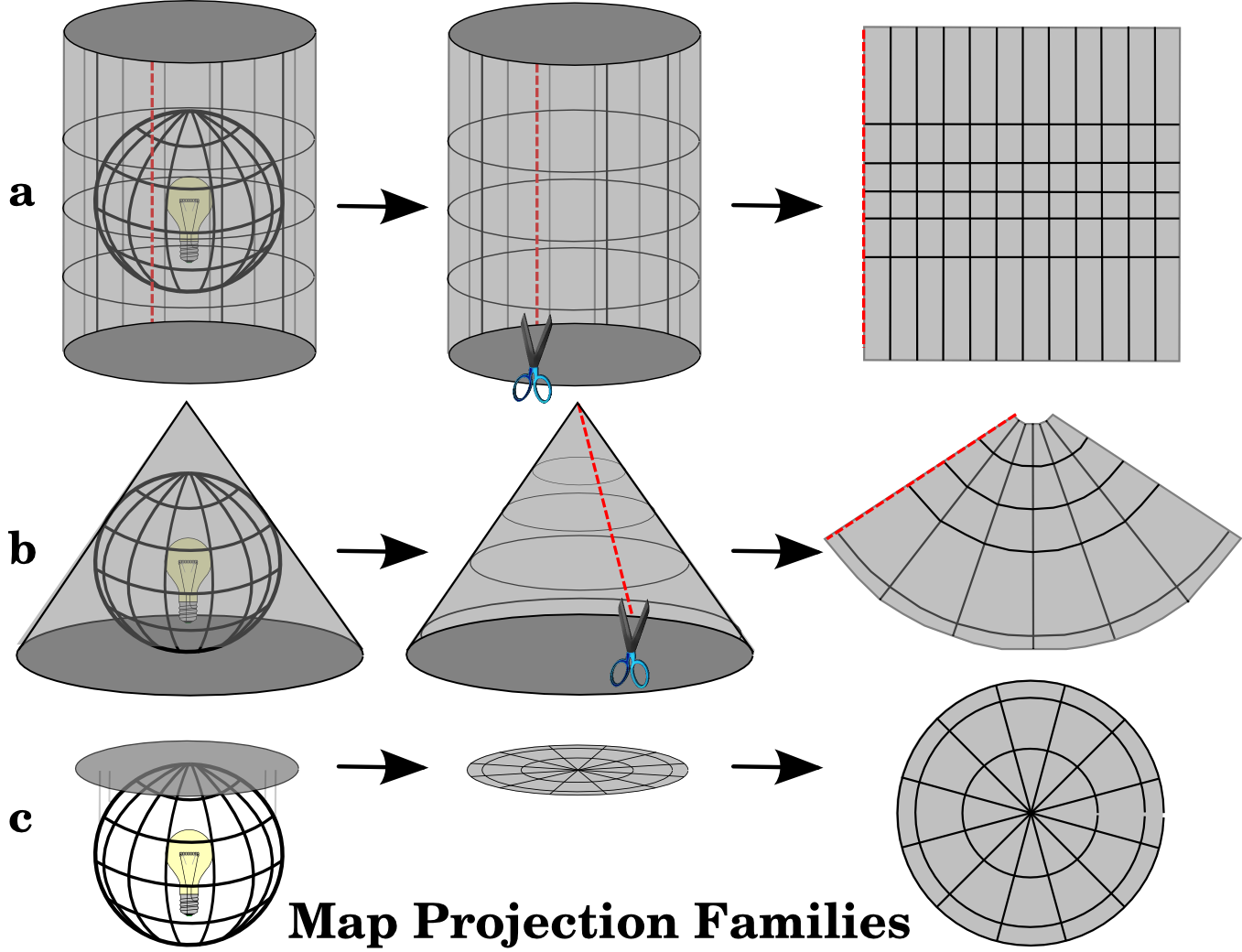
Fig. 8.3 Os três tipos de projecções cartográficas. Podem ser representadas por a) projecções cilíndricas, b) projecções cónicas ou c) projecções planares.
Hoje, naturalmente, o processo de projectar uma terra esférica num papel plano é feito usando princípios matemáticos de geometria e trigonometria, reproduzindo-se a projecção física de luz através do globo.
8.4. Precisão das projecções cartográficas
Map projections are never absolutely accurate representations of the spherical earth. As a result of the map projection process, every map shows distortions of angular conformity, distance and area. A map projection may combine several of these characteristics, or may be a compromise that distorts all the properties of area, distance and angular conformity, within some acceptable limit. Examples of compromise projections are the Winkel Tripel projection and the Robinson projection (see Fig. 8.4), which are often used for producing and visualizing world maps.
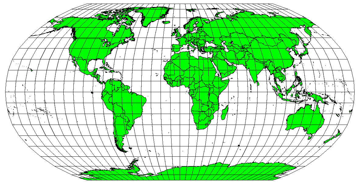
Fig. 8.4 A projecção de Robinson é um compromisso entre distorções de área, ângulo e direcção, e distância que são aceitáveis.
É geralmente impossível preservar todas as características em simultâneo numa projecção cartográfica. Isto significa que quando queremos executar operações analíticas precisas necessitamos de usar uma projecção cartográfica que fornece as melhores características para as nossas análises. Por exemplo, se for necessário medir distâncias no nosso mapa, devemos usar uma projecção que garante uma elevada precisão nas distâncias.
8.4.1. Projecções cartográficas com conformidade angular
Ao trabalhar com um globo, as principais direcções da rosa dos ventos (Norte, Este, Sul e Oeste) ocorrerão sempre a 90º umas das outras. Por outras palavras, Este ocorrerá sempre num ângulo de 90º com a direcção Norte. As propriedades angulares correctas podem ser preservadas numa projecção. Uma projecção que mantém ângulos e direcções é designada de projecção conforme ou projecção ortomórfica.
These projections are used when the preservation of angular relationships is important. They are commonly used for navigational or meteorological tasks. It is important to remember that maintaining true angles on a map is difficult for large areas and should be attempted only for small portions of the earth. The conformal type of projection results in distortions of areas, meaning that if area measurements are made on the map, they will be incorrect. The larger the area the less accurate the area measurements will be. Examples are the Mercator projection (as shown in Fig. 8.5) and the Lambert Conformal Conic projection. The U.S. Geological Survey uses a conformal projection for many of its topographic maps.
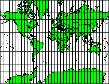
Fig. 8.5 A projecção de Mercator, por exemplo, é usada quando relações angulares são importantes, mas as relações entre áreas são distorcidas.
8.4.2. Projecções cartográficas com distâncias equivalentes
If your goal in projecting a map is to accurately measure distances, you should select a projection that is designed to preserve distances well. Such projections, called equidistant projections, require that the scale of the map is kept constant. A map is equidistant when it correctly represents distances from the centre of the projection to any other place on the map. Equidistant projections maintain accurate distances from the centre of the projection or along given lines. These projections are used for radio and seismic mapping, and for navigation. The Plate Carree Equidistant Cylindrical (see Fig. 8.6) and the Equirectangular projection are two good examples of equidistant projections. The Azimuthal Equidistant projection is the projection used for the emblem of the United Nations (see Fig. 8.7).
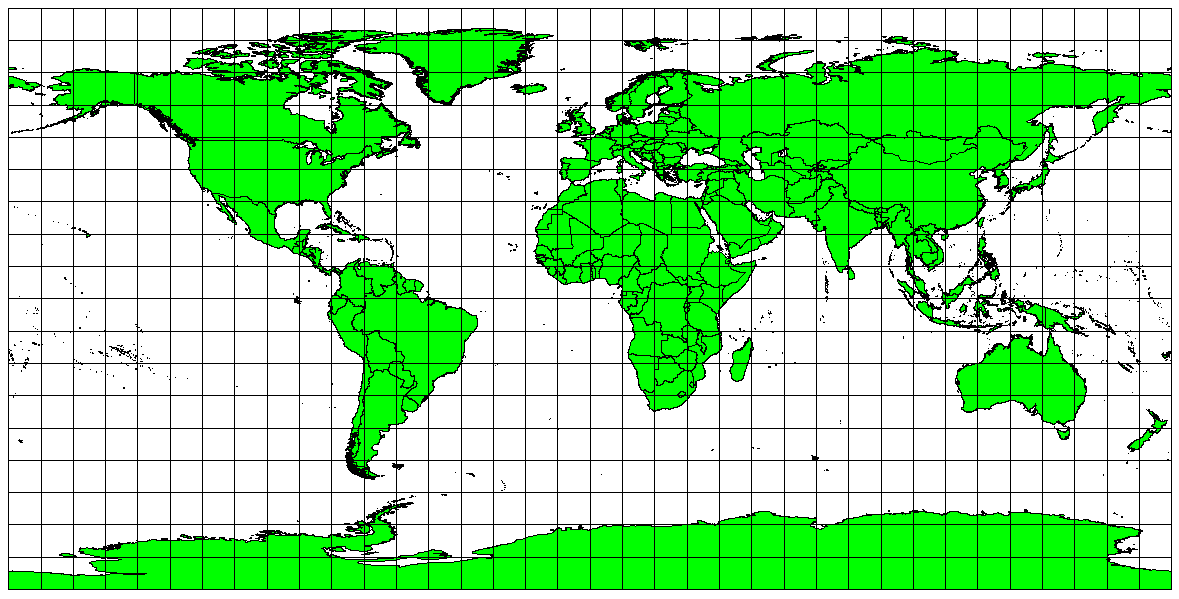
Fig. 8.6 A projecção Cilíndrica Equidistante de Plate Carree, por exemplo, é usada quando a medição precisa de distâncias é importante.

Fig. 8.7 O Logo das Nações Unidas usa a projecção Equidistante Azimutal.
8.4.3. Projecções com áreas equivalentes
When a map portrays areas over the entire map, so that all mapped areas have the same proportional relationship to the areas on the Earth that they represent, the map is an equal area map. In practice, general reference and educational maps most often require the use of equal area projections. As the name implies, these maps are best used when calculations of area are the dominant calculations you will perform. If, for example, you are trying to analyse a particular area in your town to find out whether it is large enough for a new shopping mall, equal area projections are the best choice. On the one hand, the larger the area you are analysing, the more precise your area measures will be, if you use an equal area projection rather than another type. On the other hand, an equal area projection results in distortions of angular conformity when dealing with large areas. Small areas will be far less prone to having their angles distorted when you use an equal area projection. Alber’s equal area, Lambert’s equal area and Mollweide Equal Area Cylindrical projections (shown in Fig. 8.8) are types of equal area projections that are often encountered in GIS work.
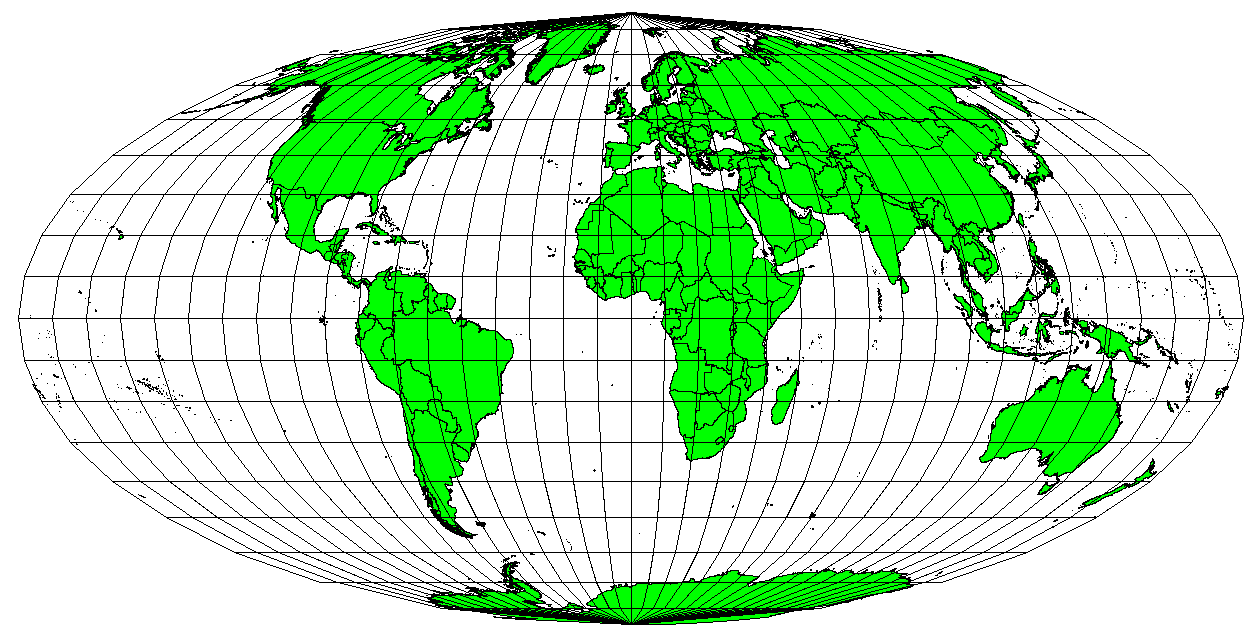
Fig. 8.8 A projecção Cilíndrica Equivalente de Mollweide, por exemplo, garante que todas as áreas cartografas têm a mesma relação proporcional com as áreas na Terra.
Tenha em atenção que as projecções cartográficas são um tópico muito complexo. Existem centenas de diferentes projecções disponíveis em todo o mundo, cada tentando retratar uma certa porção da superfície da terra o mais fielmente possível num pedaço plano de papel. Na realidade, a escolha de qual a projecção a usar será frequentemente estará já tomada. A maioria dos países têm as suas projecções mais comuns e quando informação é trocada, em geral segue-se a norma nacional.
8.5. Sistemas de Coordenadas (SC) em detalhe
Com a ajuda dos sistemas de coordenadas (SC) cada lugar na terra pode ser especificado por um conjunto de 3 números, chamados coordenadas. Em geral, os SC podem ser divididos ente sistemas de coordenadas projectados (também designados por sistemas de coordenadas Cartesianas ou rectangulares) e sistemas de coordenadas geográficas.
8.5.1. Sistemas de Coordenadas Geográficas
O uso de Sistemas de Coordenadas Geográficas é muito comum. Estes usam graus de latitude e longitude e por vezes um valor de altura para descrever uma localização na superfície da terra. O mais popular é chamado WGS 84.
Lines of latitude run parallel to the equator and divide the earth into 180 equally spaced sections from North to South (or South to North). The reference line for latitude is the equator and each hemisphere is divided into ninety sections, each representing one degree of latitude. In the northern hemisphere, degrees of latitude are measured from zero at the equator to ninety at the north pole. In the southern hemisphere, degrees of latitude are measured from zero at the equator to ninety degrees at the south pole. To simplify the digitisation of maps, degrees of latitude in the southern hemisphere are often assigned negative values (0 to -90°). Wherever you are on the earth’s surface, the distance between the lines of latitude is the same (60 nautical miles). See Fig. 8.9 for a pictorial view.
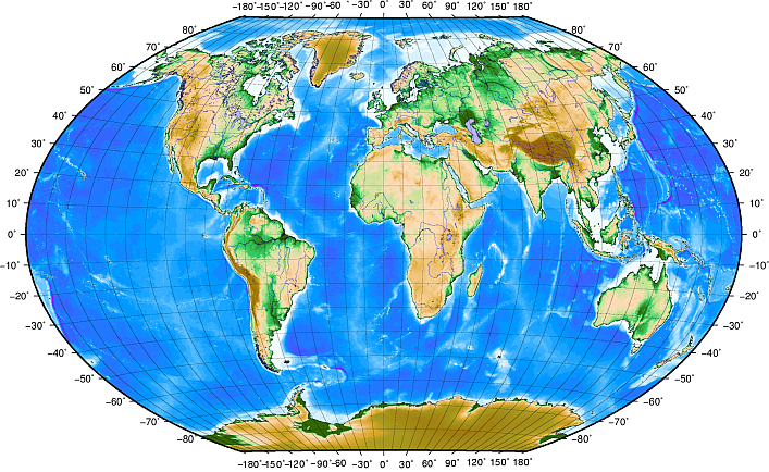
Fig. 8.9 Sistemas de coordenadas geográficas com linhas de latitude paralelas ao equador e linhas de longitude com o meridiano principal a passar por Greenwich.
Lines of longitude, on the other hand, do not stand up so well to the standard of uniformity. Lines of longitude run perpendicular to the equator and converge at the poles. The reference line for longitude (the prime meridian) runs from the North pole to the South pole through Greenwich, England. Subsequent lines of longitude are measured from zero to 180 degrees East or West of the prime meridian. Note that values West of the prime meridian are assigned negative values for use in digital mapping applications. See Fig. 8.9 for a pictorial view.
No equador, e apenas no equador, a distância representada por uma linha de longitude é igual à distância representada por um grau de latitude. Ao mover-se para os pólos, a distância entre linhas de longitude torna-se progressivamente menor, até que, na exacta localização do pólo, todos os 360º de longitude são representados por um único ponto que pode tocar com o seu dedo (quererá provavelmente usar luvas). Usando o sistema de coordenadas geográfico, podemos ter uma grelha de linhas dividindo a terra em quadrados que cobrem aproximadamente 12363,365 quilómetros quadrados até ao equador — um bom início, mas não muito útil para determinar a localização de algo num desses quadrados.
Para ser realmente útil, uma grelha no mapa deve ser dividida em secções suficientemente pequenas para que possam ser usadas para descrever (com um nível de precisão aceitável) a localização de um ponto no mapa. Para isto, graus são divididos em minutos (') e segundos ("). Existem sessenta minutos num grau, e sessenta segundos num minuto (3600 segundos num grau). Assim, no equador, um segundo de latitude ou longitude = 30,87634 metros.
8.5.2. Sistemas de coordenadas projectadas
A two-dimensional coordinate reference system is commonly defined by two axes. At right angles to each other, they form a so called XY-plane (see Fig. 8.10 on the left side). The horizontal axis is normally labelled X, and the vertical axis is normally labelled Y. In a three-dimensional coordinate reference system, another axis, normally labelled Z, is added. It is also at right angles to the X and Y axes. The Z axis provides the third dimension of space (see Fig. 8.10 on the right side). Every point that is expressed in spherical coordinates can be expressed as an X Y Z coordinate.
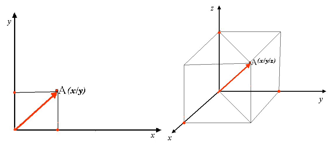
Fig. 8.10 Sistemas de coordenadas de duas e três dimensões
Um sistema de coordenadas projectadas no hemisfério sul (a sul do equador) normalmente tem a sua origem no equador numa Longitude específica. Isto significa que os valores de Y aumentam para Sul e os valores de X aumentam para Oeste. No hemisfério norte (a norte do equador) a origem é também o equador numa Longitude específica. Contudo, agora os valores de Y aumentam para Norte e os valores de X aumentam para Este. Na secção seguinte, descreveremos um sistema de coordenadas projectadas, chamado Universal Transverso de Mercator (UTM) muito usado para a África do Sul.
8.6. O SC Universal Transverso de Mercator (UTM) em detalhe
The Universal Transverse Mercator (UTM) coordinate reference system has its origin on the equator at a specific Longitude. Now the Y-values increase southwards and the X-values increase to the West. The UTM CRS is a global map projection. This means, it is generally used all over the world. But as already described in the section “accuracy of map projections” above, the larger the area (for example South Africa) the more distortion of angular conformity, distance and area occur. To avoid too much distortion, the world is divided into 60 equal zones that are all 6 degrees wide in longitude from East to West. The UTM zones are numbered 1 to 60, starting at the antimeridian (zone 1 at 180 degrees West longitude) and progressing East back to the antemeridian (zone 60 at 180 degrees East longitude) as shown in Fig. 8.11.
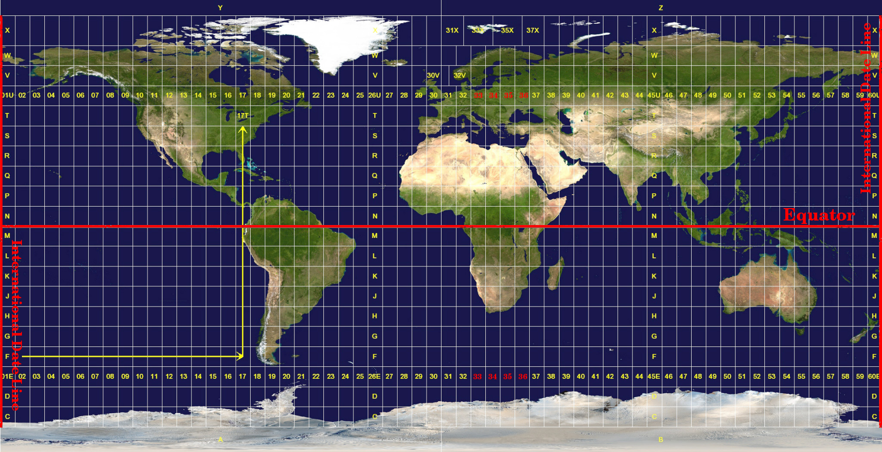
Fig. 8.11 As zonas do sistema Universal Transverso de Mercator. Para a África do Sul são usadas as zonas 33S, 34S, 35S, e 36S.
As you can see in Fig. 8.11 and Fig. 8.12, South Africa is covered by four UTM zones to minimize distortion. The zones are called UTM 33S, UTM 34S, UTM 35S and UTM 36S. The S after the zone means that the UTM zones are located south of the equator.
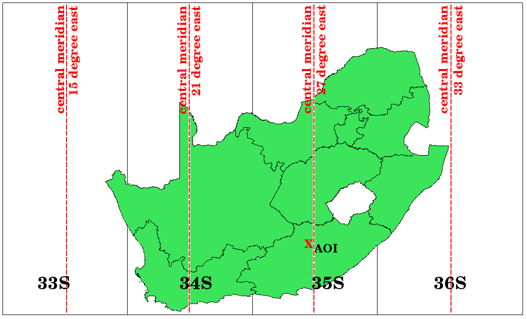
Fig. 8.12 Zonas UTM 33S, 34S, 35S, e 36S com as suas longitudes centrais (meridianos) usadas para projectar a África do Sul com alta precisão. A cruz vermelha mostra uma Área de Interesse (ADI).
Say, for example, that we want to define a two-dimensional coordinate within the Area of Interest (AOI) marked with a red cross in Fig. 8.12. You can see, that the area is located within the UTM zone 35S. This means, to minimize distortion and to get accurate analysis results, we should use UTM zone 35S as the coordinate reference system.
The position of a coordinate in UTM south of the equator must be indicated with the zone number (35) and with its northing (Y) value and easting (X) value in meters. The northing value is the distance of the position from the equator in meters. The easting value is the distance from the central meridian (longitude) of the used UTM zone. For UTM zone 35S it is 27 degrees East as shown in Fig. 8.12. Furthermore, because we are south of the equator and negative values are not allowed in the UTM coordinate reference system, we have to add a so called false northing value of 10,000,000 m to the northing (Y) value and a false easting value of 500,000 m to the easting (X) value. This sounds difficult, so, we will do an example that shows you how to find the correct UTM 35S coordinate for the Area of Interest.
8.6.1. The northing (Y) value
The place we are looking for is 3,550,000 meters south of the equator, so the northing (Y) value gets a negative sign and is -3,550,000 m. According to the UTM definitions we have to add a false northing value of 10,000,000 m. This means the northing (Y) value of our coordinate is 6,450,000 m (-3,550,000 m + 10,000,000 m).
8.6.2. The easting (X) value
First we have to find the central meridian (longitude) for the UTM zone 35S. As we can see in Fig. 8.12 it is 27 degrees East. The place we are looking for is 85,000 meters West from the central meridian. Just like the northing value, the easting (X) value gets a negative sign, giving a result of -85,000 m. According to the UTM definitions we have to add a false easting value of 500,000 m. This means the easting (X) value of our coordinate is 415,000 m (-85,000 m + 500,000 m). Finally, we have to add the zone number to the easting value to get the correct value.
Como resultado, a coordenada para o nosso Ponto de Interesse, projectado na zona UTM 35S seria escrito como: 35 415.000 m E / 6.450.000 m N. Em alguns SIG, quando a zona UTM 35S correcta é definida e as unidades escolhidas são metros, as coordenadas podem aparecer como simplesmente 415.000 6.450.000.
8.7. Projecção em Tempo-Real
Como pode provavelmente imaginar, pode surgir uma situação onde os dados que quer usar num SIG estão projectados num sistema de coordenadas diferente. Por exemplo, poderá ter um tema vectorial com os limites da África do Sul projectados em UTM 35S e outro tema vectorial de pontos com informação sobre precipitação fornecido no sistema de coordenadas geográficas WGS 84. Num SIG estes dois temas vectoriais são mostrados em duas áreas totalmente diferentes na janela do mapa, porque têm diferentes projecções.
To solve this problem, many GIS include a functionality called on-the-fly projection. It means, that you can define a certain projection when you start the GIS and all layers that you then load, no matter what coordinate reference system they have, will be automatically displayed in the projection you defined. This functionality allows you to overlay layers within the map window of your GIS, even though they may be in different reference systems. In QGIS, this functionality is applied by default.
8.8. Problemas comuns / situações a que deve estar atento
O tópico projecções cartográficas é muito complexo e até profissionais que estudaram geografia, geodesia ou outra ciência relacionada com SIG, muitas vezes têm problemas com a definição correcta de projecções cartográficas e sistemas de coordenadas. Geralmente quando trabalha com SIG, já tem dados para começar a trabalhar. Na maioria das vezes, estes dados estarão projectados num determinado SC, e não terá de criar o novo SC nem mesmo de re-projectar os dados de um SC para outro. Dito isto, é sempre útil ter uma noção do que significam projecção cartográfica e SC.
8.9. O que aprendemos?
Resumindo o que abordámos na lista seguinte:
Projecções cartográficas representam a superfície da terra num pedação de papel, ou ecrã de computador, bidimensional.
Existem projecções cartográficas globais, mas a maioria das projecções são criadas e optimizadas para áreas menores da superfície da terra.
Projecções cartográficas nunca são representações totalmente precisas da terra esférica. Mostram distorções da conformidade angular, de distâncias e de áreas. É impossível preservar todas estas características ao mesmo tempo numa projecção cartográfica.
UM Sistema de coordenadas (SC) define, com a ajuda de coordenadas, como o mapa bidimensional projectado se relaciona com locais reais na terra.
Há dois tipos diferentes de sistemas de coordenadas: Sistemas de Coordenadas Geográficas e Sistemas de Coordenadas Projectadas.
A projecção On the fly é uma funcionalidade nos SIG que permite que possa sobrepor camadas, mesmo que estejam projectadas em diferentes sistemas de referências de coordenadas.
8.10. Agora experimente!
Aqui está algumas ideias para experimentar com os seu alunos:
Start QGIS
In check No projection (or unknown/non-Earth projection)
Load two layers of the same area but with different projections
Let your pupils find the coordinates of several places on the two layers. You can show them that it is not possible to overlay the two layers.
Then define the coordinate reference system as Geographic/WGS 84 inside the Project Properties dialog
Load the two layers of the same area again and let your pupils see how setting a CRS for the project (hence, enabling «on-the-fly» projection) works.
You can open the Project Properties dialog in QGIS and show your pupils the many different Coordinate Reference Systems so they get an idea of the complexity of this topic. You can select different CRSs to display the same layer in different projections.
8.11. Algo para reflectir
If you don’t have a computer available, you can show your pupils the principles of the three map projection families. Get a globe and paper and demonstrate how cylindrical, conical and planar projections work in general. With the help of a transparency sheet you can draw a two-dimensional coordinate reference system showing X axes and Y axes. Then, let your pupils define coordinates (X and Y values) for different places.
8.12. Outras leituras
Livros:
Chang, Kang-Tsung (2006). Introduction to Geographic Information Systems. 3rd Edition. McGraw Hill. ISBN: 0070658986
DeMers, Michael N. (2005). Fundamentals of Geographic Information Systems. 3rd Edition. Wiley. ISBN: 9814126195
Galati, Stephen R. (2006): Geographic Information Systems Demystified. Artech House Inc. ISBN: 158053533X
Sítios na internet:
https://foote.geography.uconn.edu/gcraft/notes/mapproj/mapproj_f.html
http://geology.isu.edu/wapi/geostac/Field_Exercise/topomaps/index.htm
O Guia de Utilizador do |qg| também tem informação mais detalhada de como trabalhar com projecções cartográficas no |qg|.
8.13. O que vem a seguir?
Na secção que se segue nós iremos abranger mais detalhadamente a Produção de Mapas.