8. Koordinatenbezugssysteme
|
Ziele: |
Verstehen von Koordinatenbezugssystemen. |
Schlüsselwörter: |
Koordinatenbezugssysteme (KBS), Kartenprojektion, On-The-Fly-Projektion, Breitengrad, Längengrad, Hochwert, Rechtswert |
8.1. Übersicht
Map projections try to portray the surface of the earth, or a portion of the earth, on a flat piece of paper or computer screen. In layman’s term, map projections try to transform the earth from its spherical shape (3D) to a planar shape (2D).
A coordinate reference system (CRS) then defines how the two-dimensional, projected map in your GIS relates to real places on the earth. The decision of which map projection and CRS to use depends on the regional extent of the area you want to work in, on the analysis you want to do, and often on the availability of data.
8.2. Kartenprojektion im Detail
Eine traditionelle Methode zur Darstellung der Erdform ist die Nutzung von Globen. Dennoch gibt es ein Problem mit dieser Methode. Obwohl Globen den größten Teil der Erdform widerspiegeln und die räumliche Struktur der kontinent-großen Bestandteile darstellen, lassen sie sich nur sehr schwierig in der Tasche tragen. Außerdem sind sie nur für sehr kleine Maßstäbe (z.B. 1:100 Millionen) geeignet.
Die meisten thematischen Kartendaten, die in GIS-Anwendungen verwendet werden, haben bedeutend größere Maßstäbe. Typische GIS-Datensätze besitzen Maßstäbe von 1:250.000 oder größer, je nach Detailgrad. Ein Globus dieser Größe wäre sehr schwierig und teuer zu produzieren und noch schwieriger zu transportieren. Deshalb haben Kartografen eine Reihe von Techniken entwickelt namens Kartenprojektionen, die - mit angemesserer Genauigkeit - die kugelförmige Erde in zwei Dimensionen darstellen.
Von nahem betrachtet wirkt die Erde relativ flach. Aber vom Weltall aus sieht man, dass die Erde relativ kugelförmig ist. Wie wir im nächsten Thema Kartenherstellung sehen werden, sind Karten eine Widerspiegelung der Realität. Sie werden nicht nur entworfen, um Eigenschaften darzustellen, sondern auch Gestalt und räumliche Anordnung. Jede Kartenprojektion hat Vorteile und Nachteile. Die beste Kartenprojektion ist abhängig vom Maßstab der Karte und vom Verwendungszweck. Zum Beispiel könnte eine Karte inakzeptable Verzerrungen aufweisen, wenn sie für die Darstellung des gesamten afrikanischen Kontinents genutzt wird, könnte aber eine exzellente Wahl sein für eine großmaßstäbliche (detailiierte) Karte Ihres Landes. Die Eigenschaften einer Kartenprojektion können auch einige Konstruktionsmerkmale der Karte beeinflussen. Einige Projektionen sind geeignet für kleine Flächen, während andere ideal sind für Kartiergebiete mit großer Ost-West-Ausdehnung oder wieder andere für Kartiergebiete mit großer Nord-Süd-Erstreckung.
8.3. Die drei Familien der Kartenprojektionen
The process of creating map projections is best illustrated by positioning a light source inside a transparent globe on which opaque earth features are placed. Then project the feature outlines onto a two-dimensional flat piece of paper. Different ways of projecting can be produced by surrounding the globe in a cylindrical fashion, as a cone, or even as a flat surface. Each of these methods produces what is called a map projection family. Therefore, there is a family of planar projections, a family of cylindrical projections, and another called conical projections (see Abb. 8.3)
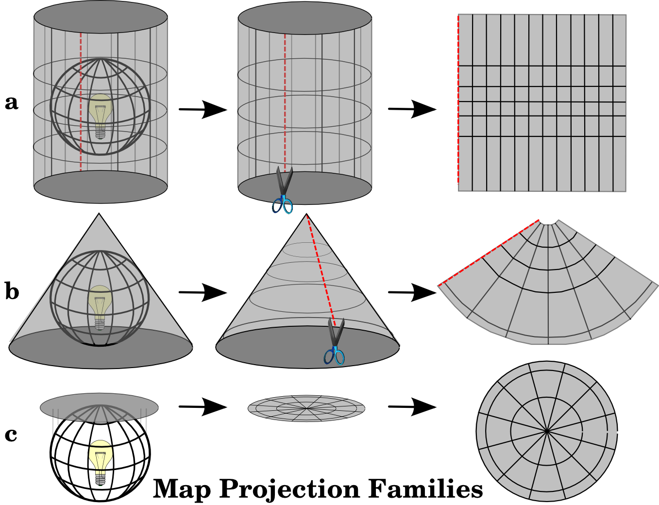
Abb. 8.3 Die drei Kategorien von Kartenprojektionen. a) Zylinderprojektion, b) Kegelprojektion und c) Azimuthalprojektion.
Natürlich wird heutzutage der Prozess, die Erdkugel auf ein flaches Blatt Papier zu projizieren, unter Zuhilfenahme mathematischer Prinzipien aus der Geometrie und Trigonometrie durchgeführt. Dies stellt die physische Projektion von Lichtstrahlen durch den Globus nach.
8.4. Genauigkeit von Kartenprojektionen
Map projections are never absolutely accurate representations of the spherical earth. As a result of the map projection process, every map shows distortions of angular conformity, distance and area. A map projection may combine several of these characteristics, or may be a compromise that distorts all the properties of area, distance and angular conformity, within some acceptable limit. Examples of compromise projections are the Winkel Tripel projection and the Robinson projection (see Abb. 8.4), which are often used for producing and visualizing world maps.

Abb. 8.4 Die Robinson Projektion ist ein Kompromiss, bei welchem Verzerrungen der Fläche, Winkeltreue und Distanz im Durchschnitt akzeptabel sind.
Es ist in der Regel nicht möglich, alle gewünschten Eigenschaften einer Kartenprojektion gleichzeitig zu erreichen. Wenn Operationen mit einer hohen Genauigkeit ausgeführt werden sollen, muss eine Kartenprojektion verwendet werden, die die besten Ergebnisse für diese Operation liefert. Wenn z. B. Abstände in der Karte gemessen werden sollen, sollte man eine Kartenprojektion mit hoher Längengenauigkeit verwenden.
8.4.1. Winkeltreue Kartenprojektionen
Wenn man mit einem Globus arbeitet, liegen die Hauptrichtungen des Kompasses (Nord, Ost, Süd und West) immer in einem Winkel von 90 Grad zueinander. Das bedeutet, dass Ost immer in einem Winkel von 90 Grad zu Nord liegt. Die Beibehaltung der korrekten Winkel kann auch mit einer Kartenprojektion erreicht werden. Eine Kartenprojektion die die Winkel richtig abbildet wird konforme Abbildung oder winkeltreue Abbildung genannt.
These projections are used when the preservation of angular relationships is important. They are commonly used for navigational or meteorological tasks. It is important to remember that maintaining true angles on a map is difficult for large areas and should be attempted only for small portions of the earth. The conformal type of projection results in distortions of areas, meaning that if area measurements are made on the map, they will be incorrect. The larger the area the less accurate the area measurements will be. Examples are the Mercator projection (as shown in Abb. 8.5) and the Lambert Conformal Conic projection. The U.S. Geological Survey uses a conformal projection for many of its topographic maps.
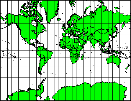
Abb. 8.5 Die Mercator Projektion wird beispielsweise benutzt, wenn Winkeltreue wichtig ist, aber Flächen verzerrt dargestellt werden dürfen.
8.4.2. Längentreue Kartenprojektionen
If your goal in projecting a map is to accurately measure distances, you should select a projection that is designed to preserve distances well. Such projections, called equidistant projections, require that the scale of the map is kept constant. A map is equidistant when it correctly represents distances from the centre of the projection to any other place on the map. Equidistant projections maintain accurate distances from the centre of the projection or along given lines. These projections are used for radio and seismic mapping, and for navigation. The Plate Carree Equidistant Cylindrical (see Abb. 8.6) and the Equirectangular projection are two good examples of equidistant projections. The Azimuthal Equidistant projection is the projection used for the emblem of the United Nations (see Abb. 8.7).
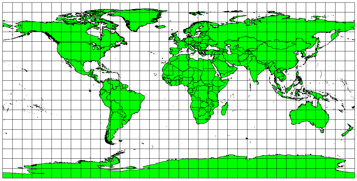
Abb. 8.6 Die Plate-Carree-Projektion wird z.B. verwendet, wenn eine genaue Längenmessung wichtig ist.

Abb. 8.7 Das Logo der Vereinten Nationen (UN) benutzt eine azimutale äquidistante Projektion.
8.4.3. Flächentreue Projektionen
When a map portrays areas over the entire map, so that all mapped areas have the same proportional relationship to the areas on the Earth that they represent, the map is an equal area map. In practice, general reference and educational maps most often require the use of equal area projections. As the name implies, these maps are best used when calculations of area are the dominant calculations you will perform. If, for example, you are trying to analyse a particular area in your town to find out whether it is large enough for a new shopping mall, equal area projections are the best choice. On the one hand, the larger the area you are analysing, the more precise your area measures will be, if you use an equal area projection rather than another type. On the other hand, an equal area projection results in distortions of angular conformity when dealing with large areas. Small areas will be far less prone to having their angles distorted when you use an equal area projection. Alber’s equal area, Lambert’s equal area and Mollweide Equal Area Cylindrical projections (shown in Abb. 8.8) are types of equal area projections that are often encountered in GIS work.
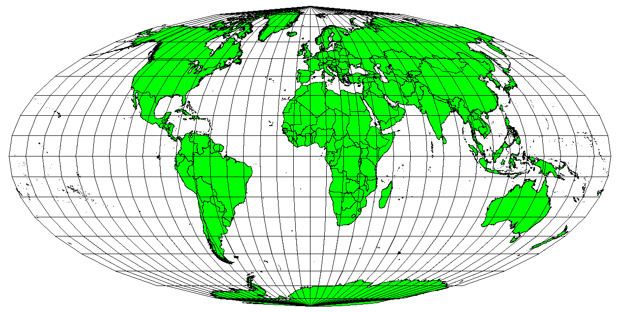
Abb. 8.8 Die Mollweide-Projektion stellt z.B. sicher, dass alle in der Karte dargstellten Flächen im selben Verhältnis zur zugehörigen Fläche auf der Erdoberfläche stehen.
Bedenken Sie, dass Kartenprojektion ein sehr komplexes Themengebiet ist. Es gibt hunderte verschiedener Projektionen weltweit, wobei jede versucht, einen bestimmten Teil der Erdoberfläche möglichst getreu auf einem ebenen Blatt Papier abzubilden. In der Realität wird einem die Wahl der Projektion oft abgenommen. In den meisten Ländern sind bestimmte Projektionen weit verbreitet. Beim Datenaustausch folgen die Leute in der Regel diesem nationalen Trend.
8.5. Koordinatenbezugssystem (KBS) im Detail
Mit Hilfe von Koordinatenbezugssystemen (KBS) kann jeder Ort auf der Erde durch eine Gruppe von drei Zahlen, genannt Koordinaten, beschrieben werden. Im Allgemeinen können KBS in projizierte Koordinatenbezugssysteme (auch kartesische oder rechtwinklige Koordinatenbezugssysteme genannt) und geographische Koordinatenbezugssysteme unterteilt werden.
8.5.1. Geografisches Koordinatensystem
Die Nutzung von geographischen Koordinatenbezugssystemen ist weit verbreitet. Sie verwenden Breiten- und Längengrade und manchmal Höhenwerte, um die Lage auf der Erdoberfläche zu beschreiben. Das beliebteste nennt sich WGS 84.
Lines of latitude run parallel to the equator and divide the earth into 180 equally spaced sections from North to South (or South to North). The reference line for latitude is the equator and each hemisphere is divided into ninety sections, each representing one degree of latitude. In the northern hemisphere, degrees of latitude are measured from zero at the equator to ninety at the north pole. In the southern hemisphere, degrees of latitude are measured from zero at the equator to ninety degrees at the south pole. To simplify the digitisation of maps, degrees of latitude in the southern hemisphere are often assigned negative values (0 to -90°). Wherever you are on the earth’s surface, the distance between the lines of latitude is the same (60 nautical miles). See Abb. 8.9 for a pictorial view.
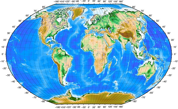
Abb. 8.9 Das geographische Koordinatenenbezugssystem mit Linien der Breitengrade, die parallel zum Äquator verlaufen und Linien der Längengrade und dem Hauptmeridian durch Greenwich.
Lines of longitude, on the other hand, do not stand up so well to the standard of uniformity. Lines of longitude run perpendicular to the equator and converge at the poles. The reference line for longitude (the prime meridian) runs from the North pole to the South pole through Greenwich, England. Subsequent lines of longitude are measured from zero to 180 degrees East or West of the prime meridian. Note that values West of the prime meridian are assigned negative values for use in digital mapping applications. See Abb. 8.9 for a pictorial view.
Nur am Äquator ist der Abstand zwischen zwei Längengraden gleich dem Abstand zwischen zwei Breitengraden. Wenn man sich in Richtung der Pole bewegt, wird der Abstand zwischen den Längengraden immer kleiner. An den Polen werden alle 360° Längengrade durch einen Punkt repräsentiert auf den man seinen Finger halten kann (man sollte dazu aber lieber Handschuhe anziehen). Das geographische Koordinatenbezugssystem unterteilt die Erdoberfläche in ein Gitter aus Vierecken, die am Äquator in etwa eine Fläche von 12363,365 Quadratkilometern erreichen. Ein guter Anfang, aber nicht ausreichend genau, um die Lage eines Objektes innerhalb solch eines Vierecks anzugeben.
Um wirklich nützlich zu sein, muss das Gitter weiter unterteilt werden, um damit die Lage eines Punktes auf der Karte (mit einer akzeptablen Genauigkeit) zu beschreiben. Um das zu erreichen, wird die Angabe Grad weiter unterteilt in Minuten (') und Sekunden ("). Es gibt sechzig Minuten in einem Grad und sechzig Sekunden in einer Minute (3600 Sekunden in einem Grad). Das bedeutet, dass am Äquator eine Längen- oder Breitensekunde einer Strecke von 30,87624 Metern entspricht.
8.5.2. Projizierte Koordinatenreferenzsysteme
A two-dimensional coordinate reference system is commonly defined by two axes. At right angles to each other, they form a so called XY-plane (see Abb. 8.10 on the left side). The horizontal axis is normally labelled X, and the vertical axis is normally labelled Y. In a three-dimensional coordinate reference system, another axis, normally labelled Z, is added. It is also at right angles to the X and Y axes. The Z axis provides the third dimension of space (see Abb. 8.10 on the right side). Every point that is expressed in spherical coordinates can be expressed as an X Y Z coordinate.
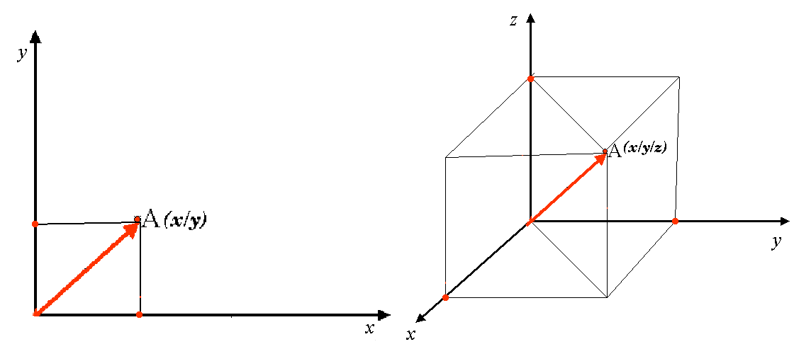
Abb. 8.10 Zwei- und dreidimensionale Koordinatenreferenzsysteme.
Ein projiziertes Koordinatenbezugssystem auf der Südhalbkugel (südlich des Äquators) hat nomalerweise seinen Ursprung an einem bestimmten Längengrad auf dem Äquator. Das bedeutet, dass die Y-Werte nach Süden und die X-Werte nach Westen anwachsen. Auf der Nordhalbkugel (nördlich des Äquators) liegt der Koordinatenursprung ebenfalls bei einem bestimmten Längengrad auf dem Äquator. Allerdings steigen die Y-Werte jetzt nordwärts und die X-Werte ostwärts an. Im folgenden Kapitel betrachte wir das projizierte Koordinatenbezugssystem Universal Transversal Mercator (UTM), das oft in Südafrika verwendet wird.
8.6. Das Universale Transversale Mercator (UTM) Koordinatensystem im Detail
The Universal Transverse Mercator (UTM) coordinate reference system has its origin on the equator at a specific Longitude. Now the Y-values increase southwards and the X-values increase to the West. The UTM CRS is a global map projection. This means, it is generally used all over the world. But as already described in the section ‚accuracy of map projections‘ above, the larger the area (for example South Africa) the more distortion of angular conformity, distance and area occur. To avoid too much distortion, the world is divided into 60 equal zones that are all 6 degrees wide in longitude from East to West. The UTM zones are numbered 1 to 60, starting at the antimeridian (zone 1 at 180 degrees West longitude) and progressing East back to the antemeridian (zone 60 at 180 degrees East longitude) as shown in Abb. 8.11.
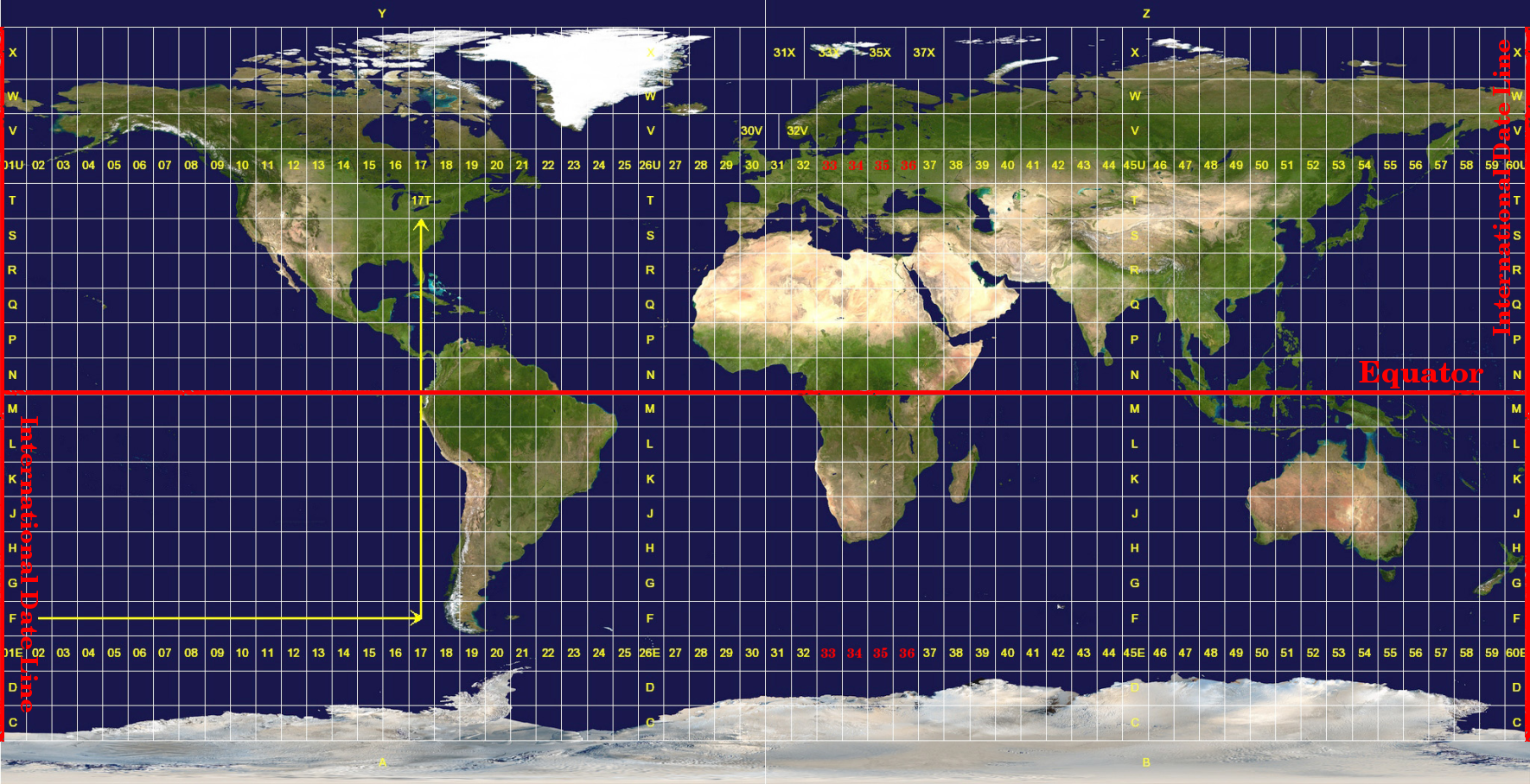
Abb. 8.11 Die Universal Transveral Mercator Zonen. Für Südafrika werden die UTM Zonen 33S, 34S, 35S und 36S genutzt.
As you can see in Abb. 8.11 and Abb. 8.12, South Africa is covered by four UTM zones to minimize distortion. The zones are called UTM 33S, UTM 34S, UTM 35S and UTM 36S. The S after the zone means that the UTM zones are located south of the equator.
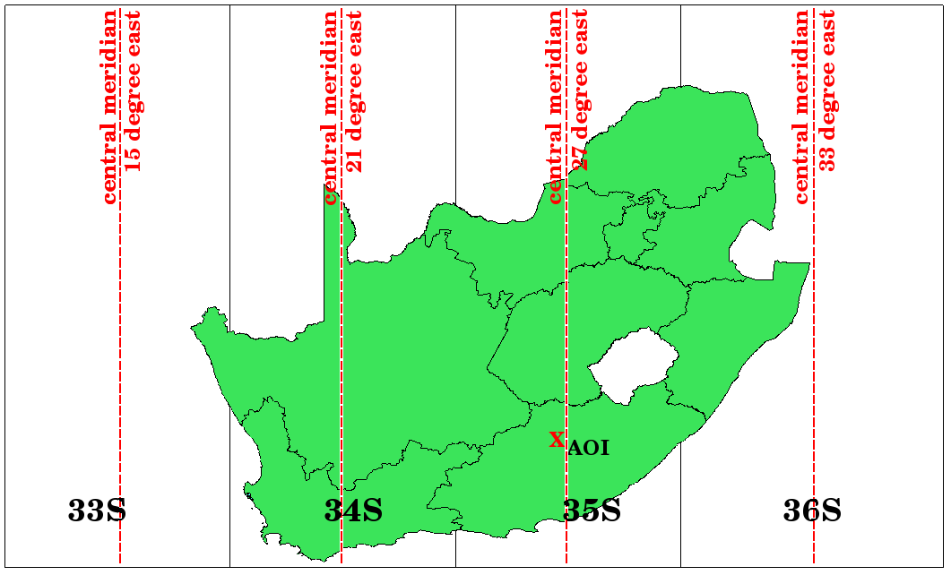
Abb. 8.12 UTM Zonen 33S, 34S, 35S und 36S mit ihren zentralen Längengraden (Meridianen), die zur hochgenauen Projektion für Südafrika verwendet werden. Das rote Kreuz zeigt ein Untersuchungsgebiet.
Say, for example, that we want to define a two-dimensional coordinate within the Area of Interest (AOI) marked with a red cross in Abb. 8.12. You can see, that the area is located within the UTM zone 35S. This means, to minimize distortion and to get accurate analysis results, we should use UTM zone 35S as the coordinate reference system.
The position of a coordinate in UTM south of the equator must be indicated with the zone number (35) and with its northing (Y) value and easting (X) value in meters. The northing value is the distance of the position from the equator in meters. The easting value is the distance from the central meridian (longitude) of the used UTM zone. For UTM zone 35S it is 27 degrees East as shown in Abb. 8.12. Furthermore, because we are south of the equator and negative values are not allowed in the UTM coordinate reference system, we have to add a so called false northing value of 10,000,000 m to the northing (Y) value and a false easting value of 500,000 m to the easting (X) value. This sounds difficult, so, we will do an example that shows you how to find the correct UTM 35S coordinate for the Area of Interest.
8.6.1. Der Hochwert (Y)
Das Untersuchungsgebiet liegt 3.550.000 südlich des Äquators. Der Hochwert (Y) erhält daher ein negatives Vorzeichen: -3.550.000 m. Entsprechend der UTM Vorgabe müssen wir den Offset für den Hochwert in Höhe von 10.000.000 m dazu addieren. Das bedeutet, dass der Hochwert (Y) unserer Koordinate 6.450.000 m (-3.550.000 m + 10.000.000 m) beträgt.
8.6.2. Der Rechtswert (X)
First we have to find the central meridian (longitude) for the UTM zone 35S. As we can see in Abb. 8.12 it is 27 degrees East. The place we are looking for is 85,000 meters West from the central meridian. Just like the northing value, the easting (X) value gets a negative sign, giving a result of -85,000 m. According to the UTM definitions we have to add a false easting value of 500,000 m. This means the easting (X) value of our coordinate is 415,000 m (-85,000 m + 500,000 m). Finally, we have to add the zone number to the easting value to get the correct value.
Im Ergebnis lautet die Koordinate unseres Point of Interest projiziert im System UTM Zone 35S: 35 415.000 m O / 6.450.000 m N. In einigen GIS werden die Koordinaten einfach als 415.000 6.450.000 angezeigt, wenn die richtige UTM Zone 35S eingestellt ist und als Einheit Meter verwendet werden.
8.7. Spontane Reprojektion / On-The-Fly Projektion
Wie man sich wahrscheinlich denken kann, gibt es Situationen in denen die im GIS zu verwendenden Daten in verschiedenen Koordinatenbezugssystemen vorliegen. Man erhält z.B. einen Vektorlayer mit der Grenze Südafrikas im projizierten System UTM 35S und einen weiteren Vektorlayer mit Punktinformationen zum Niederschlag im geographischen Koordinatensystem WGS 84. Im GIS liegen diese zwei Vektorlayer in völlig verschiedenen Bereichen des Kartenfensters, da sie verschiedene Projektionen verwenden.
To solve this problem, many GIS include a functionality called on-the-fly projection. It means, that you can define a certain projection when you start the GIS and all layers that you then load, no matter what coordinate reference system they have, will be automatically displayed in the projection you defined. This functionality allows you to overlay layers within the map window of your GIS, even though they may be in different reference systems. In QGIS, this functionality is applied by default.
8.8. Bekannte Probleme / womit man rechnen muss
Die Thematik Kartenprojektion ist sehr komplex und selbst Profis die Geographie, Geodäsie oder eine andere GIS bezogene Wissenschaft studiert haben, haben oftmals Probleme mit der korrekten Definition der Kartenprojektion und des Koordinatenbezugssystems. In der Regel liegen für die Arbeit mit GIS bereits projizierte Daten vor. In den meisten Fällen werden diese Daten in ein bestimmtes KBS projiziert, so dass man in der Regel kein neues KBS anlegen oder die Daten in eine anderes KBS reprojizieren muss. Nichts desto trotz ist es sinnvoll, eine Vorstellung davon zu haben, was Kartenprojektion und KBS bedeuten.
8.9. Was haben wir gelernt?
Lassen Sie uns zusammenfassen, was wir in diesem Arbeitsblatt behandelt haben:
Kartenprojektionen stellen die Erdoberfläche auf einem ebenen zweidimensionalen Papierstück oder Computerbildschirm dar.
Es gibt Kartenprojektionen für die gesamte Erdoberfläche, aber die meisten Projektionen sind entworfen und optimiert, um kleinere Gebiete zu projizieren.
Kartenprojektionen sind niemals eine völlig korrekte Repräsentation der kugelförmigen Erde. Sie zeigen Verzerrungen in Winkeln, Abständen und Flächen. Es ist in einer Kartenprojektion unmöglich, alle diese Eigenschaften gleichzeit zu erhalten.
Ein Koordinatenbezugssystem (KBS) bestimmt mit Hilfe von Koordinaten, wie sich eine zweidimensionale projizierte Karte zu den tatsächlichen Orten auf der Erdoberfläche verhält.
Es gibt zwei verschiedene Arten von Koordinatenbezugssystemen: geographische Koordinatensysteme und projizierte Koordinatensysteme.
Die Projektion zur Laufzeit ist eine GIS-Funktionalität, die es uns erlaubt, Layer in verschiedenen projizierten Koordinatenbezugssystemen übereinander zu legen.
8.10. Versuchen Sie es selbst!
Hier sind einige Ideen für Sie, die Sie mit Ihren Lernenden versuchen sollten:
Start QGIS
In check No projection (or unknown/non-Earth projection)
Load two layers of the same area but with different projections
Let your pupils find the coordinates of several places on the two layers. You can show them that it is not possible to overlay the two layers.
Then define the coordinate reference system as Geographic/WGS 84 inside the Project Properties dialog
Load the two layers of the same area again and let your pupils see how setting a CRS for the project (hence, enabling „on-the-fly“ projection) works.
You can open the Project Properties dialog in QGIS and show your pupils the many different Coordinate Reference Systems so they get an idea of the complexity of this topic. You can select different CRSs to display the same layer in different projections.
8.11. Etwas zum nachdenken
If you don’t have a computer available, you can show your pupils the principles of the three map projection families. Get a globe and paper and demonstrate how cylindrical, conical and planar projections work in general. With the help of a transparency sheet you can draw a two-dimensional coordinate reference system showing X axes and Y axes. Then, let your pupils define coordinates (X and Y values) for different places.
8.12. Literaturhinweise
Bücher:
Chang, Kang-Tsung (2006). Introduction to Geographic Information Systems. 3rd Edition. McGraw Hill. ISBN: 0070658986
DeMers, Michael N. (2005). Fundamentals of Geographic Information Systems. 3rd Edition. Wiley. ISBN: 9814126195
Galati, Stephen R. (2006): Geographic Information Systems Demystified. Artech House Inc. ISBN: 158053533X
Webseiten:
https://foote.geography.uconn.edu/gcraft/notes/mapproj/mapproj_f.html
http://geology.isu.edu/wapi/geostac/Field_Exercise/topomaps/index.htm
Das QGIS Benutzerhandbuch beinhält mehr Informationen zum Arbeiten mit Kartenprojektionen in QGIS.
8.13. Wie geht es weiter?
Im folgenden Abschnitt werden wir uns das Thema Kartenproduktion näher ansehen.