24.10. 外部アプリケーションの設定
プロセシングフレームワークは、追加のアプリケーションを使用して拡張できます。外部アプリケーションに依存するアルゴリズムは、独自のアルゴリズムプロバイダによって管理されます。追加のプロバイダは個別のプラグインとして見つけることができ、QGISプラグインマネージャを使用してインストールできます。
This section will show you how to configure the Processing framework to include these additional applications, and it will explain some particular features of the algorithms based on them. Once you have correctly configured the system, you will be able to execute external algorithms from any component like the toolbox or the graphical modeler, just like you do with any other algorithm.
By default, algorithms that rely on an external application not shipped with QGIS are not enabled. You can enable them in the Processing settings dialog if they are installed on your system.
24.10.1. Windowsユーザーへの注意点
If you are not an advanced user and you are running QGIS on Windows, you might not be interested in reading the rest of this chapter. Make sure you install QGIS in your system using the standalone installer. That will automatically install SAGA and GRASS in your system and configure them so they can be run from QGIS. All the algorithms from these providers will be ready to be run without needing any further configuration. If installing with the OSGeo4W application, make sure that you also select SAGA and GRASS for installation.
24.10.2. ファイルフォーマットに関する注意点
When using external software, opening a file in QGIS does not mean that it can be opened and processed in that other software. In most cases, other software can read what you have opened in QGIS, but in some cases, that might not be true. When using databases or uncommon file formats, whether for raster or vector layers, problems might arise. If that happens, try to use well-known file formats that you are sure are understood by both programs, and check the console output (in the log panel) to find out what is going wrong.
You might for instance get trouble and not be able to complete your work if you call an external algorithm with a GRASS raster layers as input. For this reason, such layers will not appear as available to algorithms.
You should, however, not have problems with vector layers, since QGIS automatically converts from the original file format to one accepted by the external application before passing the layer to it. This adds extra processing time, which might be significant for large layers, so do not be surprised if it takes more time to process a layer from a DB connection than a layer from a Shapefile format dataset of similar size.
外部アプリケーションを使用していないプロバイダーはQGISで開けるレイヤーはどれも処理できます。なぜならそれらはQGISを通じて分析のためにそれを開いているので。
All raster and vector output formats produced by QGIS can be used as input layers. Some providers do not support certain formats, but all can export to common formats that can later be transformed by QGIS automatically. As for input layers, if a conversion is needed, that might increase the processing time.
24.10.3. ベクターレイヤー選択に関する注意点
外部アプリケーションがQGIS内でベクターレイヤーに存在する選択を知らされることもできます。しかし、それにはそれらが元から外部アプリケーションでサポートされていない形式であったかのように、すべての入力ベクターレイヤーを書き換えることが必要です。選択が存在しないか、 選択された地物のみを使用 オプションが処理の一般設定で有効になっていない場合にのみ、レイヤーは外部アプリケーションに直接渡すことができます。
In other cases, exporting only selected features is needed, which causes longer execution times.
24.10.4. SAGA: System for Automated Geoscientific Analyses、地球科学自動分析システム
SAGA algorithms can be run from QGIS if SAGA is included with the QGIS installation.
If you are running Windows, both the stand-alone installer and the OSGeo4W installer include SAGA.
24.10.4.1. SAGAグリッドシステムの制限について
複数の入力ラスターレイヤーを必要とするほとんどのSAGAアルゴリズムは、それらが同じグリッド系を持つことを必要としています。つまり、それらが同じ地理的領域をカバーして同じセルサイズを持ち、対応するグリッドが一致する必要があります。QGISからSAGAアルゴリズムを呼び出すときは、そのセルサイズと範囲に関係なく、どんなレイヤーも使用できます。複数のラスターレイヤーはSAGAアルゴリズムのための入力として使用される場合、QGISは(SAGAアルゴリズムが異なるグリッド系からのレイヤーで動作できない場合)共通のグリッド系にそれらをリサンプリングした後、SAGAに渡します。
その一般的なグリッド系の定義は、ユーザーによって制御され、そうする設定ウィンドウのSAGAグループ内のいくつかのパラメーターがあります。ターゲットグリッド系を設定する2つの方法があります。
手動で設定する。次のパラメーターの値を設定することによって範囲を定義します。
リサンプリング最小X
リサンプリング最大X
リサンプリング最小Y
リサンプリング最大Y
リサンプリングセルサイズ
QGISはその範囲に対して入力レイヤーを、それらがその範囲と重複していない場合でも、再サンプリングすることに注意してください。
入力レイヤーから自動的に設定する。このオプションを選択するには、 リサンプリングにグリッド系の最小カバーを使用 オプションチェックするだけです。他のすべての設定は無視され、すべての入力レイヤーを最小でカバーする範囲が使用されます。ターゲットレイヤーのセルサイズは、入力レイヤーの全てのセルサイズの最大値です。
多重ラスターレイヤーを使用しないあるいは固有の入力グリッドシステムを必要としないアルゴリズムでは、SAGAを呼び出す前にリサンプリングは実行されませんし、これらのパラメーターは使用されません。
24.10.4.2. マルチバンドレイヤーに関する制限
QGISとは異なり、SAGAではマルチバンドレイヤーをサポートしていません。(例えばRGBまたはマルチスペクトル画像のような)マルチバンドレイヤーを使用する場合は、最初にシングルバンド化された画像に分割する必要があります。そうするためには、「SAGA/グリッドツール/RGB画像を分割」アルゴリズム(RGB画像から三つの画像を作成する)や「SAGA /グリッドツール/バンド抽出」アルゴリズム(単一バンドを抽出する)を使用できます。
24.10.4.3. セルサイズの制限
SAGAではラスターレイヤーがx軸とy軸において同じセルサイズであることを仮定しています。もし、水平方向と垂直方向でセルサイズが異なる値のレイヤーで作業するならば、予期せぬ結果を得ることになるでしょう。この場合、入力レイヤーがSAGAによって適切に処理されないであろうという警告がプロセスログに加えられることになります。
24.10.4.4. ログを記録する
QGISはSAGAを呼び出すと、それはこれにより、すべての必要な操作を実行するためにコマンドのセットを通過する、そのコマンドラインインターフェイスを使用しません。SAGAは、追加のコンテンツと共に、既に行われる処理のパーセンテージを含むコンソールに情報を書き込むことにより、その進捗状況を示しています。この出力はフィルタがかけられ、アルゴリズムの実行中に、プログレスバーを更新するために使用されます。
Both the commands sent by QGIS and the additional information printed by SAGA can be logged along with other processing log messages, and you might find them useful to track what is going on when QGIS runs a SAGA algorithm. You will find two settings, namely Log console output and Log execution commands, to activate that logging mechanism.
Most other providers that use external applications and call them through the command-line have similar options, so you will find them as well in other places in the processing settings list.
24.10.5. R scripts
To enable R in Processing you need to install the Processing R Provider plugin and configure R for QGIS.
Configuration is done in in the Processing tab of .
Depending on your operating system, you may have to use R folder to specify where your R binaries are located.
注釈
On Windows the R executable file is normally in
a folder (R-<version>) under C:\Program Files\R\.
Specify the folder and NOT the binary!
On Linux you just have to make sure that the R folder is
in the PATH environment variable.
If R in a terminal window starts R, then you are ready to go.
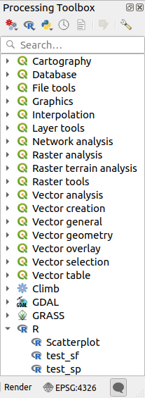
After installing the Processing R Provider plugin, you will find some example scripts in the Processing Toolbox:
Scatterplot runs an R function that produces a scatter plot from two numerical fields of the provided vector layer.
test_sf does some operations that depend on the
sfpackage and can be used to check if the R packagesfis installed. If the package is not installed, R will try to install it (and all the packages it depends on) for you, using the Package repository specified in in the Processing options. The default is https://cran.r-project.org/. Installing may take some time...test_sp can be used to check if the R package
spis installed. If the package is not installed, R will try to install it for you.
If you have R configured correctly for QGIS, you should be able to run these scripts.
24.10.5.1. Adding R scripts from the QGIS collection
R integration in QGIS is different from that of SAGA in that there is not a predefined set of algorithms you can run (except for some example script that come with the Processing R Provider plugin).
A set of example R scripts is available in the QGIS Repository. Perform the following steps to load and enable them using the QGIS Resource Sharing plugin.
Add the QGIS Resource Sharing plugin (you may have to enable Show also experimental plugins in the Plugin Manager Settings)
Open it (Plugins --> Resource Sharing --> Resource Sharing)
Choose the Settings tab
Click Reload repositories
Choose the All tab
Select QGIS R script collection in the list and click on the Install button
The collection should now be listed in the Installed tab
Close the plugin
Open the Processing Toolbox, and if everything is OK, the example scripts will be present under R, in various groups (only some of the groups are expanded in the screenshot below).
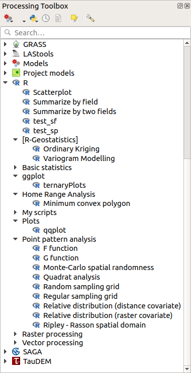
図 24.33 The Processing Toolbox with some R scripts shown
The scripts at the top are the example scripts from the Processing R Provider plugin.
If, for some reason, the scripts are not available in the Processing Toolbox, you can try to:
Open the Processing settings ( tab)
Go to
On Ubuntu, set the path to (or, better, include in the path):
/home/<user>/.local/share/QGIS/QGIS3/profiles/default/resource_sharing/repositories/github.com/qgis/QGIS-Resources/collections/rscripts
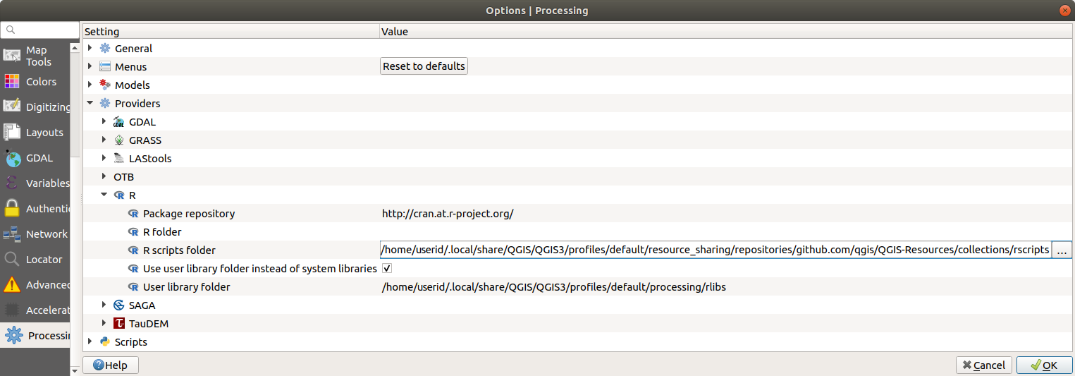
On Windows, set the path to (or, better, include in the path):
C:\Users\<user>\AppData\Roaming\QGIS\QGIS3\profiles\default\resource_sharing\repositories\github.com\qgis\QGIS-Resources\collections\rscripts
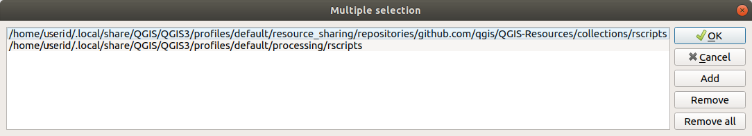
To edit, double-click. You can then choose to just paste / type the path, or you can navigate to the directory by using the ... button and press the Add button in the dialog that opens. It is possible to provide several directories here. They will be separated by a semicolon (";").
If you would like to get all the R scrips from the QGIS 2 on-line collection, you can select QGIS R script collection (from QGIS 2) instead of QGIS R script collection. You will probably find that scripts that depend on vector data input or output will not work.
24.10.5.2. Creating R scripts
You can write scripts and call R commands, as you would do from R. This section shows you the syntax for using R commands in QGIS, and how to use QGIS objects (layers, tables) in them.
To add an algorithm that calls an R function (or a more complex R script that you have developed and you would like to have available from QGIS), you have to create a script file that performs the R commands.
R script files have the extension .rsx, and creating them is
pretty easy if you just have a basic knowledge of R syntax and R
scripting.
They should be stored in the R scripts folder.
You can specify the folder (R scripts folder) in the
R settings group in Processing settings dialog).
Let’s have a look at a very simple script file, which calls the R
method spsample to create a random grid within the boundary of the
polygons in a given polygon layer.
This method belongs to the maptools package.
Since almost all the algorithms that you might like to incorporate
into QGIS will use or generate spatial data, knowledge of spatial
packages like maptools and sp/sf, is very useful.
##Random points within layer extent=name
##Point pattern analysis=group
##Vector_layer=vector
##Number_of_points=number 10
##Output=output vector
library(sp)
spatpoly = as(Vector_layer, "Spatial")
pts=spsample(spatpoly,Number_of_points,type="random")
spdf=SpatialPointsDataFrame(pts, as.data.frame(pts))
Output=st_as_sf(spdf)
The first lines, which start with a double Python comment sign
(##), define the display name and group of the script, and
tell QGIS about its inputs and outputs.
注釈
To find out more about how to write your own R scripts, have a look at the R Intro section in the training manual and consult the QGIS R Syntax section.
When you declare an input parameter, QGIS uses that information for two things: creating the user interface to ask the user for the value of that parameter, and creating a corresponding R variable that can be used as R function input.
In the above example, we have declared an input of type vector,
named Vector_layer.
When executing the algorithm, QGIS will open the layer selected
by the user and store it in a variable named Vector_layer.
So, the name of a parameter is the name of the variable that you
use in R for accessing the value of that parameter (you should
therefore avoid using reserved R words as parameter names).
Spatial parameters such as vector and raster layers are read using
the st_read() (or readOGR) and brick() (or readGDAL)
commands (you do not have to worry about adding those commands to
your description file -- QGIS will do it), and they are stored as
sf (or Spatial*DataFrame) objects.
Table fields are stored as strings containing the name of the selected field.
Vector files can be read using the readOGR() command instead
of st_read() by specifying ##load_vector_using_rgdal.
This will produce a Spatial*DataFrame object instead of an
sf object.
Raster files can be read using the readGDAL() command instead
of brick() by specifying ##load_raster_using_rgdal.
If you are an advanced user and do not want QGIS to create the
object for the layer, you can use ##pass_filenames to indicate
that you prefer a string with the filename.
In this case, it is up to you to open the file before performing
any operation on the data it contains.
With the above information, it is possible to understand the first lines of the R script (the first line not starting with a Python comment character).
library(sp)
spatpoly = as(Vector_layer, "Spatial")
pts=spsample(polyg,numpoints,type="random")
The spsample function is provided by the sp library, so
the first thing we do is to load that library.
The variable Vector_layer contains an sf object.
Since we are going to use a function (spsample) from the sp
library, we must convert the sf object to a
SpatialPolygonsDataFrame object using the as function.
Then we call the spsample function with this object and
the numpoints input parameter (which specifies the number of
points to generate).
Since we have declared a vector output named Output, we have to
create a variable named Output containing an sf object.
We do this in two steps.
First we create a SpatialPolygonsDataFrame object from the
result of the function, using the SpatialPointsDataFrame function,
and then we convert that object to an sf object using the
st_as_sf function (of the sf library).
You can use whatever names you like for your intermediate
variables.
Just make sure that the variable storing your final result has
the defined name (in this case Output), and that it contains
a suitable value (an sf object for vector layer output).
In this case, the result obtained from the spsample method had
to be converted explicitly into an sf object via a
SpatialPointsDataFrame object, since it is itself an object of
class ppp, which can not be returned to QGIS.
アルゴリズムは、ラスターレイヤーを生成した場合、それらが保存されている方法は、 ##dontuserasterpackage オプションを使用しているかどうかに依存します。それを使用している場合は、これらのレイヤーは、 writeGDAL() メソッドを使用して保存されます。そうでない場合、 raster パッケージから writeRaster() メソッドが使用されます。
If you have used the ##pass_filenames option, outputs are
generated using the raster package (with writeRaster()).
If your algorithm does not generate a layer, but a text result in
the console instead, you have to indicate that you want the
console to be shown once the execution is finished.
To do so, just start the command lines that produce the results
you want to print with the > ('greater than') sign.
Only output from lines prefixed with > are shown.
For instance, here is the description file of an algorithm that
performs a normality test on a given field (column) of the
attributes of a vector layer:
##layer=vector
##field=field layer
##nortest=group
library(nortest)
>lillie.test(layer[[field]])
最後の行の出力が印刷されているが、第一の出力はない(そしていずれも、他のコマンドラインからの出力は、QGISによって自動的に追加されています)。
If your algorithm creates any kind of graphics (using the plot()
method), add the following line (output_plots_to_html used to be
showplots):
##output_plots_to_html
これは、QGISはRの実行が完了した後に開かれる一時ファイルにすべてのRのグラフィック出力をリダイレクトするようになります。
Both graphics and console results will be available through the processing results manager.
For more information, please check the R scripts in the official QGIS collection (you download and install them using the QGIS Resource Sharing plugin, as explained elsewhere). Most of them are rather simple and will greatly help you understand how to create your own scripts.
注釈
The sf, rgdal and raster libraries are loaded by default,
so you do not have to add the corresponding library() commands.
However, other libraries that you might need have to be
explicitly loaded by typing:
library(ggplot2) (to load the ggplot2 library).
If the package is not already installed on your machine, Processing
will try to download and install it.
In this way the package will also become available in R Standalone.
Be aware that if the package has to be downloaded, the script
may take a long time to run the first time.
24.10.6. R libraries
The R script sp_test tries to load the R packages sp and
raster.
24.10.6.1. R libraries installed when running sf_test
The R script sf_test tries to load sf and raster.
If these two packages are not installed, R may try to load and install
them (and all the libraries that they depend on).
The following R libraries end up in
~/.local/share/QGIS/QGIS3/profiles/default/processing/rscripts
after sf_test has been run from the Processing Toolbox on Ubuntu with
version 2.0 of the Processing R Provider plugin and a fresh install of
R 3.4.4 (apt package r-base-core only):
abind, askpass, assertthat, backports, base64enc, BH, bit, bit64, blob, brew, callr, classInt, cli, colorspace, covr, crayon, crosstalk, curl, DBI, deldir,
desc, dichromat, digest, dplyr, e1071, ellipsis, evaluate, fansi, farver, fastmap, gdtools, ggplot2, glue, goftest, gridExtra, gtable, highr, hms,
htmltools, htmlwidgets, httpuv, httr, jsonlite, knitr, labeling, later, lazyeval, leafem, leaflet, leaflet.providers, leafpop, leafsync, lifecycle, lwgeom,
magrittr, maps, mapview, markdown, memoise, microbenchmark, mime, munsell, odbc, openssl, pillar, pkgbuild, pkgconfig, pkgload, plogr, plyr, png, polyclip,
praise, prettyunits, processx, promises, ps, purrr, R6, raster, RColorBrewer, Rcpp, reshape2, rex, rgeos, rlang, rmarkdown, RPostgres, RPostgreSQL,
rprojroot, RSQLite, rstudioapi, satellite, scales, sf, shiny, sourcetools, sp, spatstat, spatstat.data, spatstat.utils, stars, stringi, stringr, svglite,
sys, systemfonts, tensor, testthat, tibble, tidyselect, tinytex, units, utf8, uuid, vctrs, viridis, viridisLite, webshot, withr, xfun, XML, xtable
24.10.7. GRASS: Geographic Resources Analysis Support System、地理的資源分析支援システム
Configuring GRASS is not much different from configuring SAGA. First, the path to the GRASS folder has to be defined, but only if you are running Windows.
By default, the Processing framework tries to configure its GRASS connector to use the GRASS distribution that ships along with QGIS. This should work without problems for most systems, but if you experience problems, you might have to configure the GRASS connector manually. Also, if you want to use a different GRASS installation, you can change the setting to point to the folder where the other version is installed. GRASS 7 is needed for algorithms to work correctly.
If you are running Linux, you just have to make sure that GRASS is correctly installed, and that it can be run without problem from a terminal window.
GRASSアルゴリズムは、計算するための領域を使用します。この領域は、アルゴリズムを毎回実行するために使用されるすべての入力レイヤーを覆う最小範囲をとる、自動的SAGA構成に見られるものと同様の値を用いて、または手動で定義できます。後者のアプローチが好む動作である場合、GRASSの設定パラメーターで 最小カバー領域を使用 オプションをチェックするだけです。
24.10.8. LAStools
To use LAStools in QGIS, you need to download and install LAStools on your computer and install the LAStools plugin (available from the official repository) in QGIS.
On Linux platforms, you will need Wine to be able to run some of the tools.
LAStools is activated and configured in the Processing options
(, Processing tab,
), where you can specify the
location of LAStools (LAStools folder) and Wine
(Wine folder).
On Ubuntu, the default Wine folder is /usr/bin.
24.10.9. OTB Applications
OTB applications are fully supported within the QGIS Processing framework.
OTB (Orfeo ToolBox) is an image processing library for remote sensing data. It also provides applications that provide image processing functionalities. The list of applications and their documentation are available in OTB CookBook
注釈
Note that OTB is not distributed with QGIS and needs to be installed separately. Binary packages for OTB can be found on the download page.
To configure QGIS processing to find the OTB library:
Open the processing settings: (left panel)*
You can see OTB under "Providers":
Expand the OTB tab
Tick the Activate option
Set the OTB folder. This is the location of your OTB installation.
Set the OTB application folder. This is the location of your OTB applications (
<PATH_TO_OTB_INSTALLATION>/lib/otb/applications)Click "ok" to save the settings and close the dialog.
If settings are correct, OTB algorithms will be available in the Processing Toolbox.
24.10.9.1. Documentation of OTB settings available in QGIS Processing
Activate: This is a checkbox to activate or deactivate the OTB provider. An invalid OTB setting will uncheck this when saved.
OTB folder: This is the directory where OTB is available.
OTB application folder: This is the location(s) of OTB applications.
Multiple paths are allowed.
Logger level (optional): Level of logger to use by OTB applications.
The level of logging controls the amount of detail printed during algorithm execution. Possible values for logger level are
INFO,WARNING,CRITICAL,DEBUG. This value isINFOby default. This is an advanced user configuration.Maximum RAM to use (optional): by default, OTB applications use all available system RAM.
You can, however, instruct OTB to use a specific amount of RAM (in MB) using this option. A value of 256 is ignored by the OTB processing provider. This is an advanced user configuration.
Geoid file (optional): Path to the geoid file.
This option sets the value of the elev.dem.geoid and elev.geoid parameters in OTB applications. Setting this value globally enables users to share it across multiple processing algorithms. Empty by default.
SRTM tiles folder (optional): Directory where SRTM tiles are available.
SRTM data can be stored locally to avoid downloading of files during processing. This option sets the value of elev.dem.path and elev.dem parameters in OTB applications. Setting this value globally enables users to share it across multiple processing algorithms. Empty by default.
24.10.9.2. Compatibility between QGIS and OTB versions
All OTB versions (from OTB 6.6.1) are compatible with the latest QGIS version.
24.10.9.3. Troubleshoot
If you have issues with OTB applications in QGIS Processing, please open an issue
on the OTB bug tracker,
using the qgis label.
Additional information about OTB and QGIS can be found here