重要

翻訳はあなたが参加できるコミュニティの取り組みです。このページは現在 100.00% 翻訳されています。

17.5. さらなるアルゴリズムとデータタイプ

注釈

このレッスンでは、さらに3つのアルゴリズムを実行し、他の入力タイプを使用する方法を学習し、出力が指定したフォルダに自動的に保存されるように設定します。

このレッスンにはひとつのテーブルとひとつのポリゴンレイヤが必要です。テーブル内の座標に基づいてポイントレイヤを作成し、各ポリゴン内のポイントの数を数えます。このレッスンに対応するQGISプロジェクト(second_alg)を開くと、XとY座標を持ったテーブルがありますが、ポリゴンレイヤはありませんが心配しないでください。これからプロセシング・ジオアルゴリズムを使って作成します。

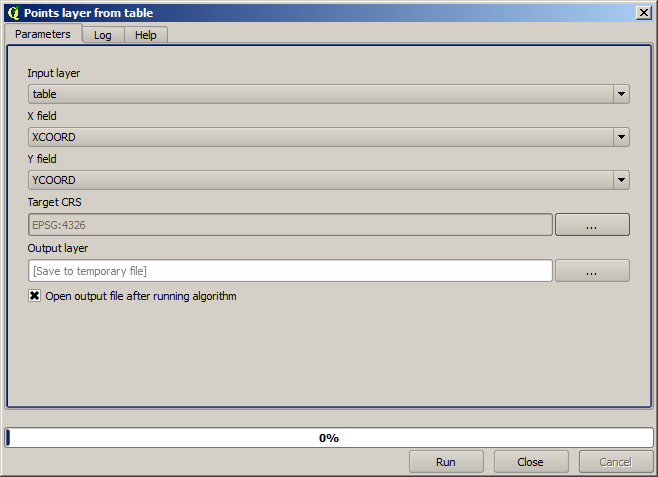
まずやることは、 テーブルから点レイヤを作成 アルゴリズムを使用して、テーブル内の座標からポイントレイヤを作成することです。もう検索ボックスの使い方は知っているので、それを見つけるのは難しくない筈です。それをダブルクリックして実行し、次のダイアログを表示させます。

このアルゴリズムは、前のレッスンのようにただ1つの出力を生成し、また、3つの入力を持っています：

テーブル ：座標を持つテーブル。ここでレッスンのデータからテーブルを選択する必要があります。
XとYフィールド ：これら2つのパラメータは最初のものに関連しています。対応するセレクタには、選択したテーブルで利用できるフィールドの名前が表示されます。 X パラメータには XCOORD フィールド、 Y パラメータには YYCOORD フィールドを選択してください。
CRS ：このアルゴリズムでは入力レイヤに何も取らないので、それに基づいたCRSを出力レイヤへ割り当てることができません。代わりに、テーブルの座標に使われているCRSを手動で選択するように求められます。左側のボタンをクリックして QGIS CRSセレクタを開き、出力CRSとしてEPSG:4326を選択してください。テーブル内の座標がそのCRSなので、このCRSを使用しています。

ダイアログは次のようになります。

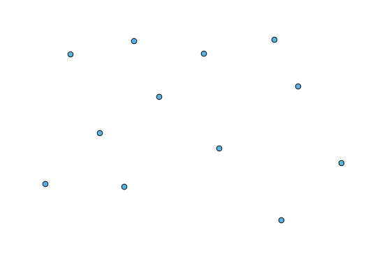
次に実行ボタンを押して、次のレイヤを得ます（新たに作成されたポイントの周辺にマップを再表示するにはズームを最大にする必要があるかもしれません）:

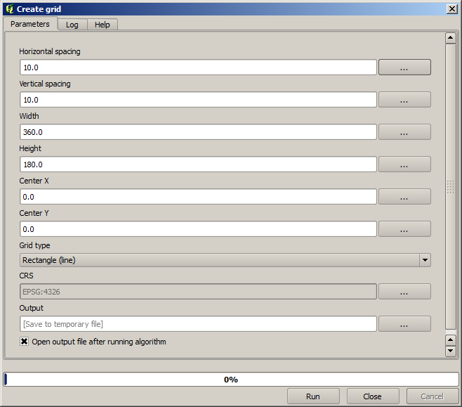
次に必要とするのはポリゴンレイヤです。グリッドを作成 アルゴリズムを使用して、構造格子のポリゴンを作成します。このアルゴリズムには次のパラメータダイアログがあります。

警告

QGISの最近のバージョンではオプションが単純になりました。XとYの最小値と最大値を入力するだけです（推奨値：-5.696226, -5.695122, 40.24742, 40.248171）

グリッドを作成するために必要な入力はすべて数値です。数値を入力する必要がある場合、次の2つのオプションがあります: 対応するボックスに直接入力するか、右にあるボタンをクリックして次のようなダイアログボックスを表示させます。

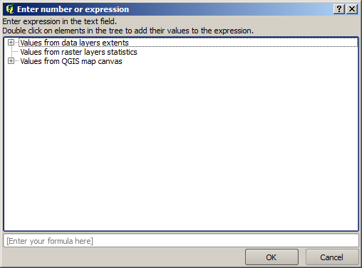
このダイアログには簡単な計算機が含まれており、 11 * 34.7 + 4.6 のような式を入力すると、計算結果がパラメータダイアログの対応するテキストボックスに入ります。また、それには定数や利用可能な他のレイヤの値も含んでいます。

ここでは入力ポイントレイヤの範囲を覆うグリッドを作成したいので、それらの座標を使い、アルゴリズムがグリッドを作成するのに要するパラメータであるグリッドの中心座標と幅と高さを計算する必要があります。少し数学が必要ですが、計算機ダイアログと入力ポイントレイヤの定数を使って自分でやってみましょう。

グリッドタイプ フィールドは 長方形（ポリゴン） を選択します。

最後のアルゴリズムの場合のように、ここにもCRSを入力する必要があります。前に行ったように、ターゲットCRSとしてEPSG:4326を選択します。

最終的に、次のようなパラメータダイアログになるはずです:

../../../_images/graticule_parameters.png

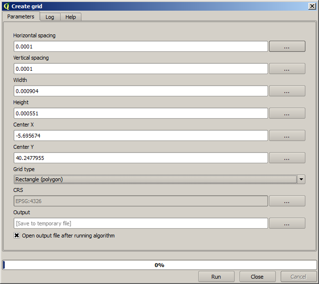
（幅と高さにひとつ間隔を追加した方が良いでしょう：水平間隔：0.0001、垂直間隔：0.0001、幅：0.001004、高さ：0.000651、中心X：-5.695674、中心Y：40.2477955）X中心は少し複雑です: -5.696126 +（（-5.695222+ 5.696126）/ 2）

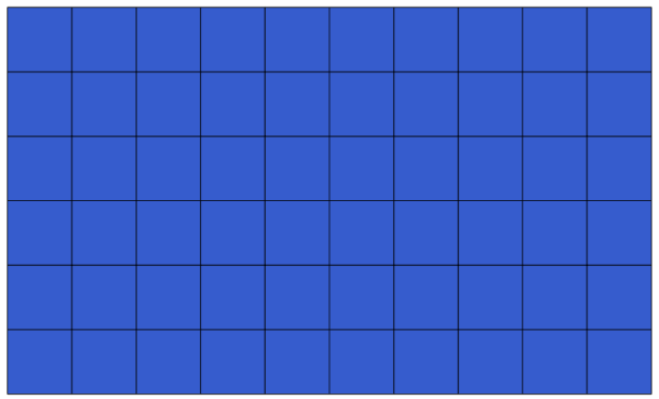
実行を押すと経緯線網レイヤが表示されます。

最後のステップは、その経緯線網の各長方形の中の点を数えることです。 ポリゴン内の点の数 アルゴリズムを使用します。

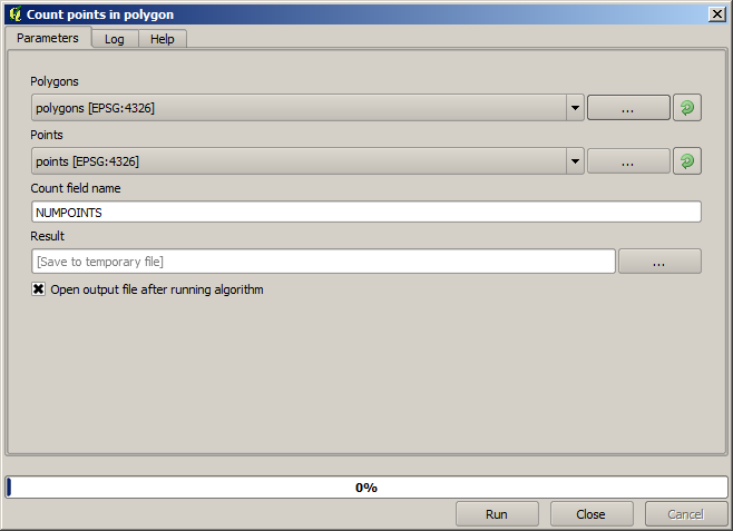
これで求めていた結果が得ることができました。

このレッスンを終える前に、データを永続的に保存したい場合に役立つ簡単なヒントを紹介します。全ての出力ファイルを特定のフォルダに保存したい場合、フォルダ名を毎回入力する必要はありません。代わりに、プロセシングメニューに移動し、 オプションと設定 を選択します。すると設定ダイアログが開きます。

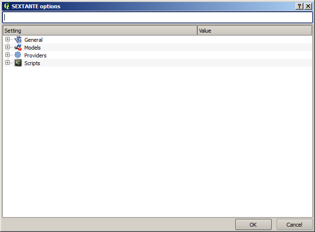
一般情報 グループで見つかる 出力フォルダ エントリで、保存先フォルダのパスを入力します。

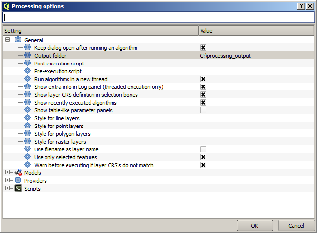
これでアルゴリズムを実行するときに、完全パスの代わりにファイル名を使うだけでよくなりました。例えば上の設定において、先ほどのアルゴリズムの出力パスとして graticule.shp を入力すると、結果は D:\processing_output\graticule.shp に保存されます。結果を別のフォルダに保存したい場合は、完全パスを入力することもできます。

グリッドを作成 アルゴリズムを異なるグリッドサイズで、またグリッドの異なる種類で自分で試してみてください。