重要
翻訳は あなたが参加できる コミュニティの取り組みです。このページは現在 100.00% 翻訳されています。
17.15. ラスタレイヤをクリッピングしてマージする
注釈
このレッスンでは、現実の世界のシナリオで地理アルゴリズムを継続して使用する、空間データの準備の別の例が表示されます。
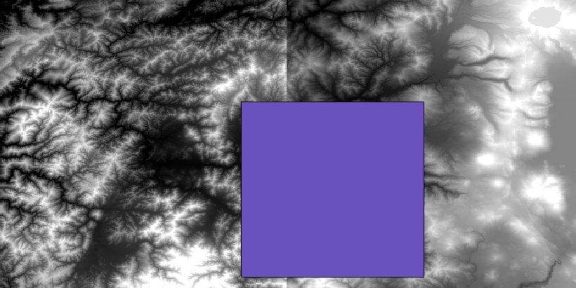
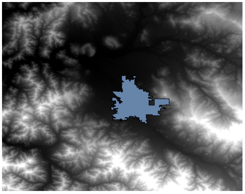
このレッスンでは、市街地を囲む領域の傾斜レイヤを計算します。領域は単独のポリゴンを持ったベクタレイヤで与えられます。ベースDEMは2つのラスタレイヤに分割されており、合わせると作業したい都市の周りよりはるかに大きい領域をカバーしています。このレッスンに対応したプロジェクトを開くと、次のように表示されます。
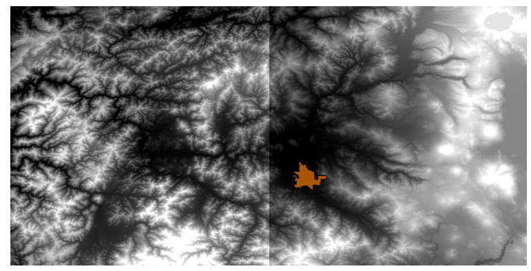
これらのレイヤには二つの問題があります。
それらは欲しいものより広過ぎる領域をカバーしています(興味があるのは市の中心部周辺のより小さな領域です)
それらは2つの異なるファイルにあります(市域は1つだけのラスタレイヤに入るが、言った通り、その周りにいくつかの余分な面積が欲しい)。
それらの両方が適切な地理アルゴリズムで簡単に解決できます。
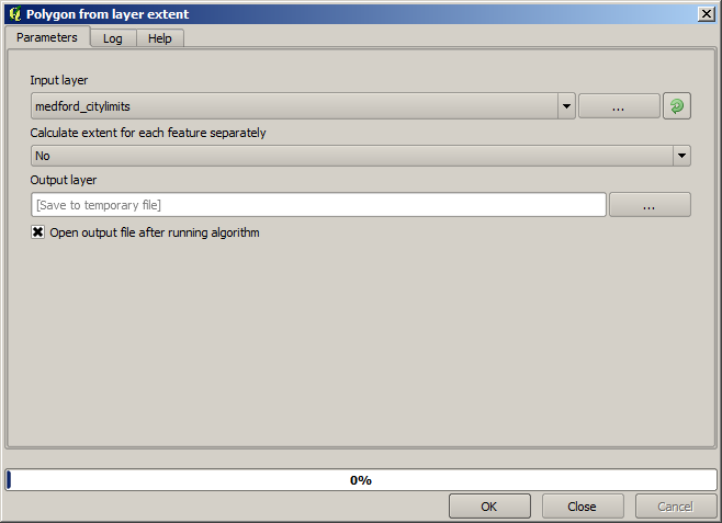
まず、欲しい領域を定義する矩形を作成します。これを行うには、市の領域の際を有するレイヤのバウンディングボックスを含むレイヤを作成し、次にそれをバッファリングして、厳密に必要であるより少し大きくカバーするラスタレイヤが得られるようにします。
バウンディングボックスを計算するために、 レイヤ範囲を抽出 アルゴリズムを使用できます
それをバッファリングするために、以下のパラメータ値で バッファ アルゴリズムを使用します。
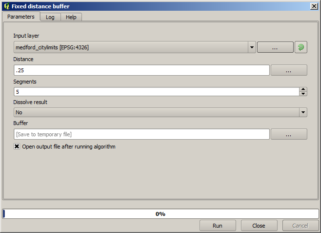
警告
構文は最近のバージョンで変更されました;距離とアークの頂点の両方を0.25に設定します
これが上に示したパラメーターを用いて得られた結果のバウンディングボックスです
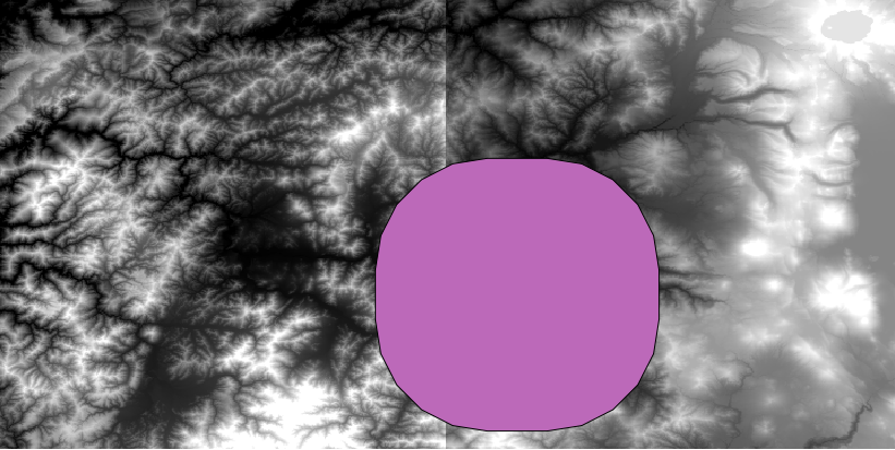
これは丸みを帯びたボックスですが、それに レイヤ範囲を抽出 アルゴリズムを実行することで、正方形の角度での同等のボックスを簡単に取得できます。市の境界を先にバッファリングして、範囲矩形を計算することでひとつのステップを省略できたでしょう。
そのラスタはベクタと異なる投影法を有していることに気づきます。したがって先に進む前に、 ワープ(再投影) ツールを使って、それらを再投影する必要があります。
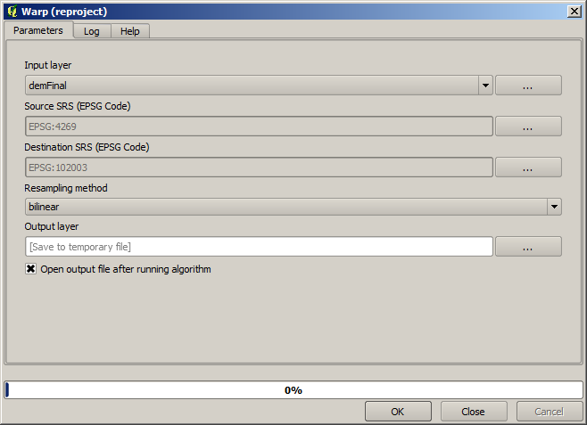
注釈
最近のバージョンではより複雑なインターフェイスになっています。少なくとも1つの圧縮方式が選択されていることを確認します。
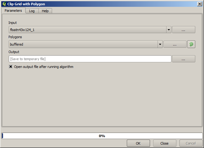
入手したいラスタレイヤのバウンディングボックスを含んでいるこのレイヤを、 ポリゴンでラスタをクリップ アルゴリズムに使用して、両方のラスタレイヤを切り出すことができます。
レイヤを切り出したら、SAGA Mosaic raster layers アルゴリズムを使ってレイヤをマージすることができます。
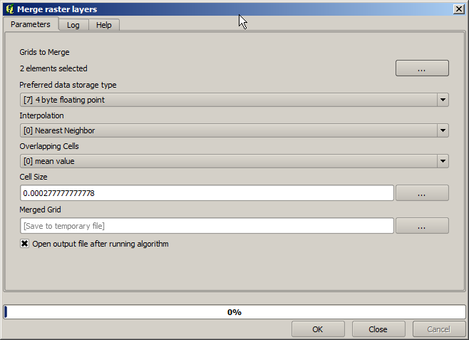
注釈
最初にマージしてから切り出しすると時間を節約でき、クリッピングアルゴリズムを二回呼び出さずにすみます。しかしながら、マージするレイヤが複数あってそれらがかなり大きなサイズの場合、それが後工程に処理が困難であるよりも大きなレイヤになってしまいます。その場合はクリッピングアルゴリズムを複数回呼び出す必要があるかもしれず、それには時間がかかるかもしれません。でも心配しないでください。その操作を自動化するためのいくつかの追加のツールがあることがすぐに分かりますから。この例ではレイヤは二つだけなので、今それを心配することはありません。
それによって、私たちが望む最後のDEMが得られます。
では傾斜レイヤを計算しましょう。
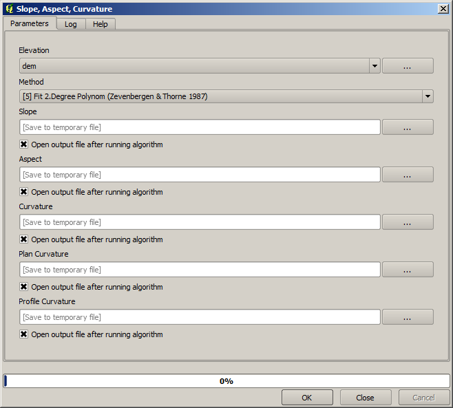
傾斜レイヤは 傾斜 アルゴリズムを用いて計算できますが、最後の工程で得られたDEMは、標高値はメートル単位でもセルサイズはメートル単位で表現されていないため、入力として適していません(レイヤは地理座標を持つCRSを使用しています)。再投影が必要です。ラスタレイヤを再投影するために、再び ワープ(再投影) アルゴリズムが使用できます。単位にメートルを持つCRS(例えば3857)に再投影し、その後、SAGAかGDALのどちらかで傾斜を正しく計算できます。
新DEMでは、傾きが計算できるようになりました。
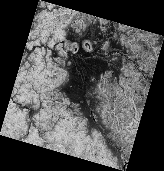
そして、これが結果の傾斜レイヤです。
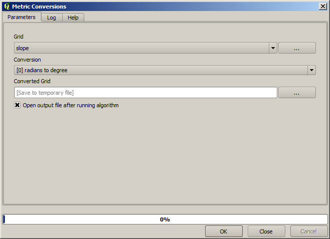
傾斜 アルゴリズムによって作成された傾斜は、度またはラジアンで表現できます。度は、より実用的で一般的な単位です。ラジアンで計算した場合は、 メトリック変換 アルゴリズムが変換するのに役立ちます(しかし、そのアルゴリズムが存在していることを知らなかった場合は、すでに使ったラスタ計算機を使用できたでしょう)。
ラスタレイヤ再投影 を使って変換された斜面レイヤを再投影して戻すと、望んでいた最終レイヤが得られます。
再投影プロセスでは、最初のステップの1つで計算されたバウンディングボックス外のデータを最終レイヤが格納するようにしている可能性があります。これは、ベースDEMを得るためにしたのと同じように、それを再びクリッピングすることによって解決できます。