Important
翻译是一项社区工作 你可以加入。此页面目前翻译进度为 59.26%。
17.5. 更多算法与数据类型
Note
本课程中,我们将运行三个新算法,学习如何使用其他输入类型,并配置输出结果自动保存到指定文件夹。
本课程需要一个表格和一个多边形图层。我们将根据表格中的坐标创建点图层,然后统计每个多边形内的点数。如果您打开本课程对应的 QGIS 项目,会发现一个包含 X 和 Y 坐标的表格,但没有多边形图层。请不用担心,我们将使用一个处理地理算法来创建它。
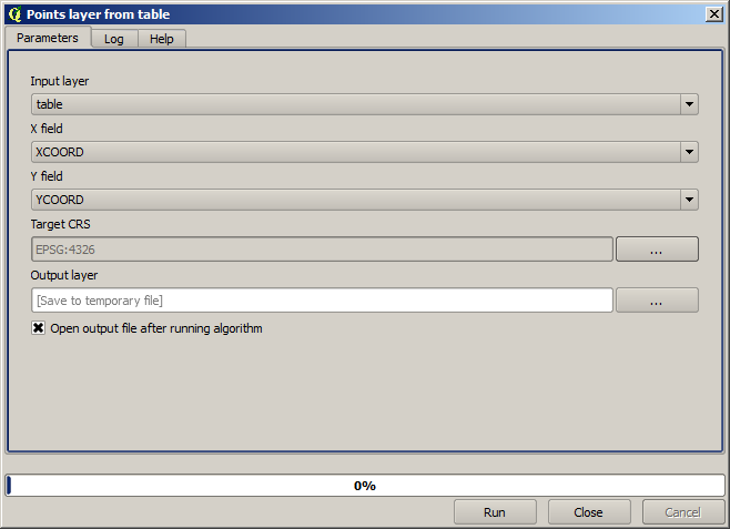
The first thing we are going to do is to create a points layer from the coordinates in the table, using the Create points layer from table algorithm. You now know how to use the search box, so it should not be hard for you to find it. Double-click on it to run it and get to its following dialog.
与上一课程的算法类似,此算法仅生成一个输出,包含三个输入参数:
*Table*(表格):包含坐标的表格。请在此选择课程数据中的表格。
X and Y fields: these two parameters are linked to the first one. The corresponding selector will show the name of those fields that are available in the selected table. Select the
XCOORDfield for the X parameter, and theYCOORDfield for the Y parameter.CRS:由于此算法不接受输入图层,无法据此自动设置输出图层的 CRS,因此需手动指定表格中坐标所使用的 CRS。点击左侧按钮打开 QGIS CRS 选择器,选择 EPSG:4326 作为输出 CRS。我们使用此 CRS 是因为表格中的坐标采用的就是该坐标系。
您的对话框应如下图所示。
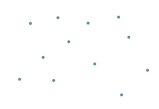
Now press the Run button to get the following layer (you may need to zoom full to reenter the map around the newly created points):
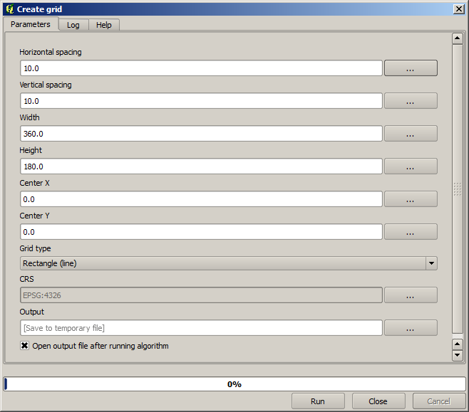
The next thing we need is the polygon layer. We are going to create a regular grid of polygons using the Create grid algorithm, which has the following parameters dialog.
Warning
在较新版本的 QGIS 中,选项更为简化;您只需输入 X 和 Y 的最小值与最大值(建议值:-5.696226, -5.695122, 40.24742, 40.248171)。
创建格网所需的输入均为数值。输入数值时,您有两种选择:直接在对应框中键入,或点击右侧按钮打开如下所示的对话框。
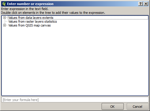
该对话框内置简易计算器,您可输入如 11 * 34.7 + 4.6 的表达式,计算结果将自动填入参数对话框的对应文本框中。此外,它还提供可用的常量及其他图层的数值。
此处,我们希望创建一个覆盖输入点图层范围的格网,因此应利用点图层的坐标计算格网的中心坐标、宽度和高度——这些正是算法创建格网所需的参数。请尝试结合计算器对话框及点图层提供的常量,自行完成这些计算。
Select Rectangles (polygons) in the Grid type field.
与上一个算法类似,此处也需指定 CRS。请如前所述,选择 EPSG:4326 作为目标 CRS。
最终,您的参数对话框应如下图所示:
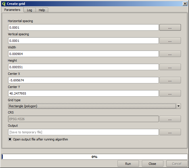
(Better add one spacing on the width and height: Horizontal spacing: 0.0001, Vertical spacing: 0.0001, Width: 0.001004, Height: 0.000651, Center X: -5.695674, Center Y: 40.2477955)
The case of X center is a bit tricky, see: -5.696126+(( -5.695222+ 5.696126)/2)
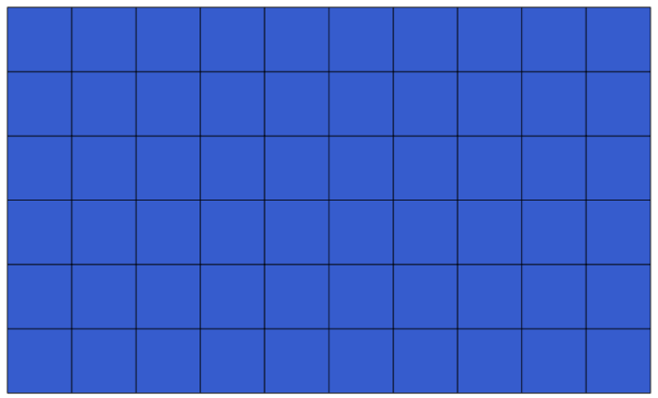
Press Run and you will get the graticule layer.
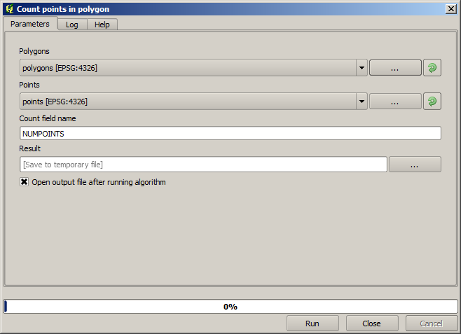
The last step is to count the points in each one of the rectangles of that graticule. We will use the Count points in polygons algorithm.
现在,我们已获得所需的结果。
在结束本课程前,提供一个便捷技巧:如果您希望持久化保存数据,可将所有输出文件统一保存到指定文件夹,而无需每次输入路径。请进入处理(Processing)菜单,选择 选项与配置 项,打开配置对话框。(3.40版本集成在,设置->选项->数据处理)
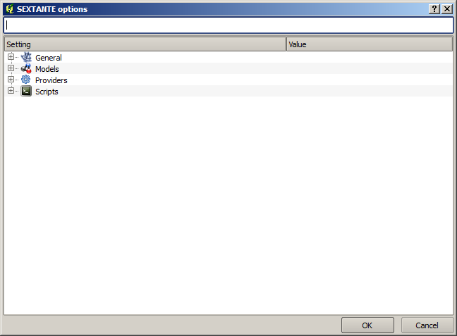
In the Output folder entry that you will find in the General group, type the path to your destination folder.
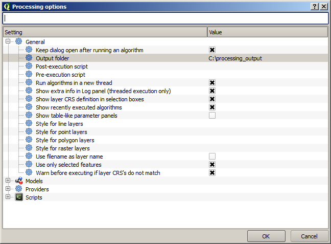
Now when you run an algorithm, just use the filename instead of the full path. For instance, with the configuration shown above, if you enter graticule.shp as the output path for the algorithm that we have just used, the result will be saved in D:processing_outputgraticule.shp. You can still enter a full path in case you want a result to be saved in a different folder.
Try yourself the Create grid algorithm with different grid sizes, and also with different types of grids.