17.16. Análise hidrológica

Nota

En esta lección vamos a realizar algunos análisis hidrológicos. Este análisis será utilizado en algunas de las siguientes lecciones, como se constituye un muy buen ejemplo de un flujo de trabajo de análisis, y lo utilizaremos para mostrar algunas características avanzadas.

Objectives: Starting with a DEM, we are going to extract a channel network, delineate watersheds and calculate some statistics.

1. Lo primero es cargar el proyecto con los datos de la lección, que solo contiene un MDT.

   

2. The first module to execute is Catchment area (in some SAGA versions it is called Flow accumulation (Top Down)). You can use any of the others named Catchment area. They have different algorithms underneath, but the results are basically the same.

3. Select the DEM in the Elevation field, and leave the default values for the rest of the parameters.

   

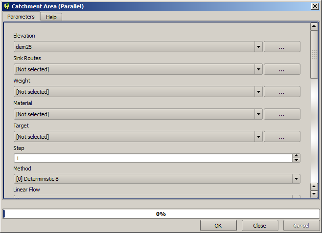
   Some algorithms calculate many layers, but the Catchment Area layer is the only one we will be using. You can get rid of the other ones if you want.

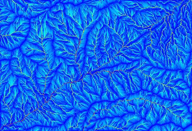
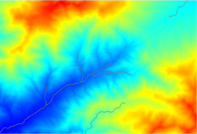
   El renderizado de la capa no es muy informativa.

   

   To know why, you can have a look at the histogram and you will see that values are not evenly distributed (there are a few cells with very high value, those corresponding to the channel network). Use the Raster calculator algorithm to calculate the logarithm of the catchment value area and you will get a layer with much more information

   

4. The catchment area (also known as flow accumulation) can be used to set a threshold for channel initiation. This can be done using the Channel network algorithm.

   • Initiation grid: use the catchment area layer and not the logarithm one.

   • Initiation threshold: 10.000.000

   • Initiation type: Greater than

   

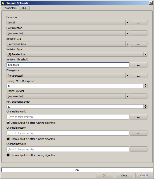
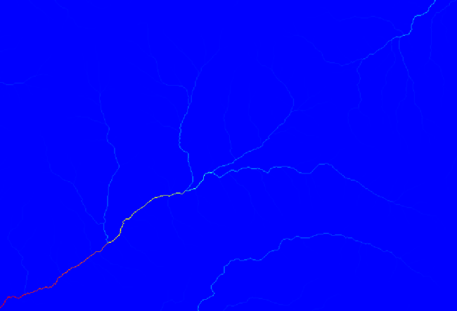
   If you increase the Initiation threshold value, you will get a more sparse channel network. If you decrease it, you will get a denser one. With the proposed value, this is what you get.

   

   The image above shows just the resulting vector layer and the DEM, but there should be also a raster layer with the same channel network. That raster will be, in fact, the layer we will be using.

5. Now, we will use the Watersheds basins algorithm to delineate the subbasins corresponding to that channel network, using as outlet points all the junctions in it. Here is how you have to set the corresponding parameters dialog.

   

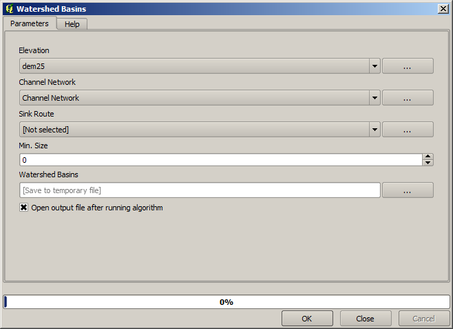
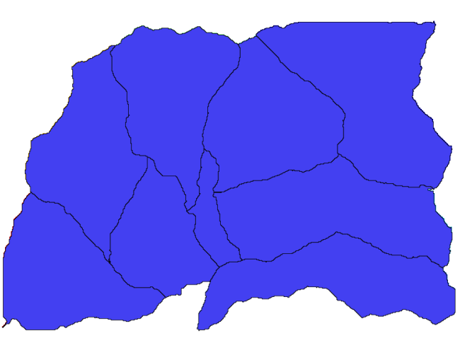
   Y esto es lo que obtendrá.

   

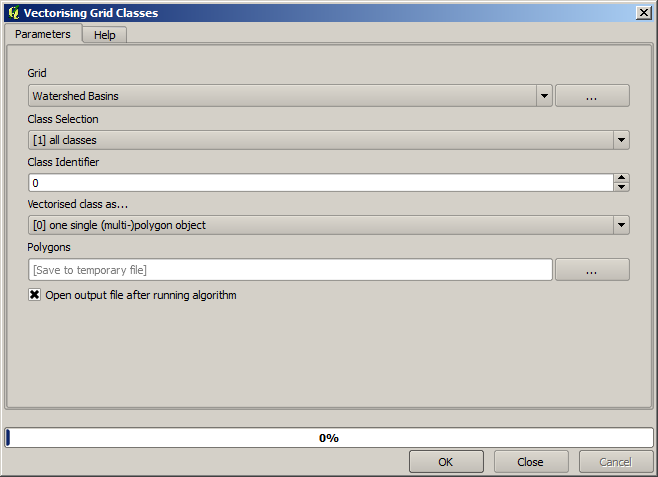
6. This is a raster result. You can vectorise it using the Vectorising grid classes algorithm.

   

   

Ahora, vamos a tratar de calcular estadísticas sobre los valores de elevación en una de las subcuencas. La idea es tener una capa que simplemente represente la elevación dentro de esa subcuenca y luego pasarla al módulo que calcula estas estadísticas.

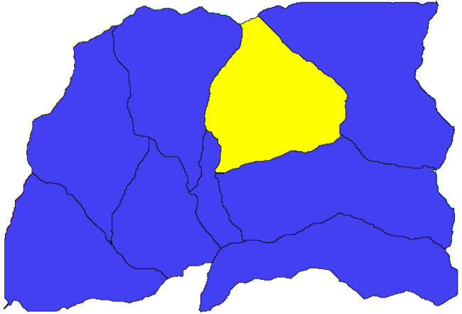
1. First, let’s clip the original DEM with the polygon representing a subbasin. We will use the Clip raster with polygon algorithm. If we select a single subbasin polygon and then call the clipping algorithm, we can clip the DEM to the area covered by that polygon, since the algorithm is aware of the selection.

   1. Select a polygon

      

   2. Call the clipping algorithm with the following parameters:

      

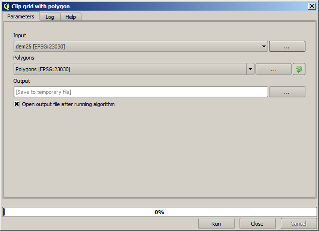
      The element selected in the input field is, of course, the DEM we want to clip.

      Obteremos algo como isto.

      

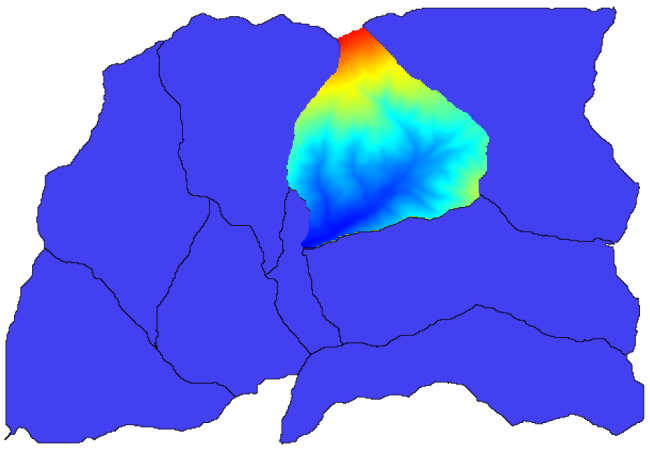
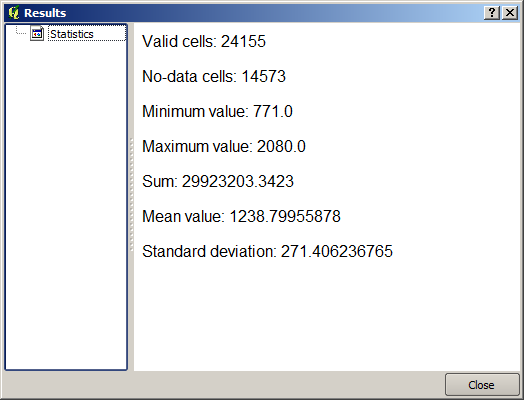
2. This layer is ready to be used in the Raster layer statistics algorithm.

   

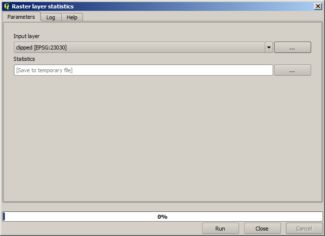
   As estatísticas resultantes são as seguintes.

   

Vamos a utilizar tanto el procedimiento de cálculo de cuenca y el cálculo de las estadísticas en otras lecciones, para averiguar cómo otros elementos pueden ayudar a automatizar ambos y trabajar más eficazmente.