17.16. 수문학적 분석

참고

이 강의에서는 수문학적 분석을 수행할 것입니다. 이 분석은 분석 작업 흐름에 대한 매우 훌륭한 예이기 때문에, 이어지는 강의들에서도 사용될 것입니다. 이 분석을 통해 몇몇 고급 기능들도 소개하겠습니다.

Objectives: Starting with a DEM, we are going to extract a channel network, delineate watersheds and calculate some statistics.

1. 먼저 이 강의에 해당하는 프로젝트를 불러오십시오. DEM 하나만을 담고 있습니다.

   

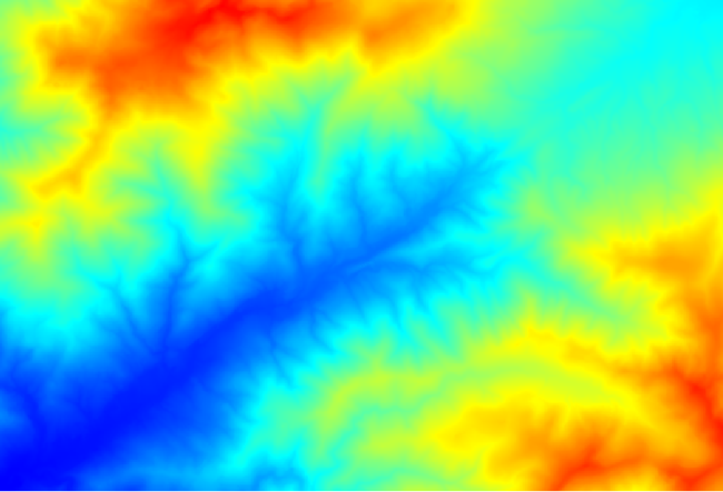
2. The first module to execute is Catchment area (in some SAGA versions it is called Flow accumulation (Top Down)). You can use any of the others named Catchment area. They have different algorithms underneath, but the results are basically the same.

3. Select the DEM in the Elevation field, and leave the default values for the rest of the parameters.

   

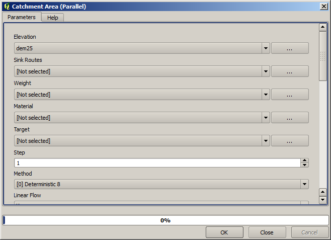
   Some algorithms calculate many layers, but the Catchment Area layer is the only one we will be using. You can get rid of the other ones if you want.

   이 레이어의 렌더링에서 그렇게 많은 정보를 알 수가 없습니다.

   

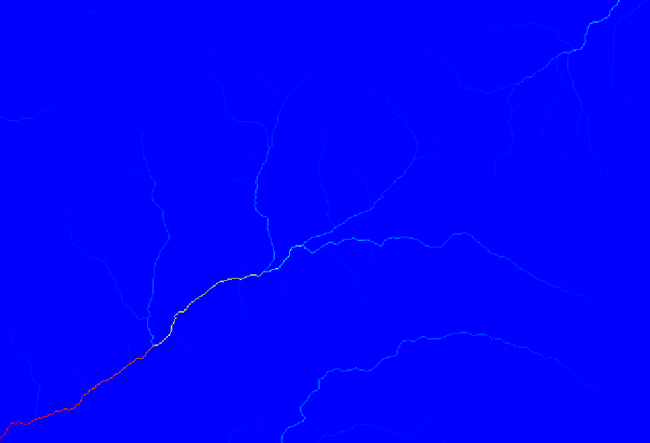
   To know why, you can have a look at the histogram and you will see that values are not evenly distributed (there are a few cells with very high value, those corresponding to the channel network). Use the Raster calculator algorithm to calculate the logarithm of the catchment value area and you will get a layer with much more information

   

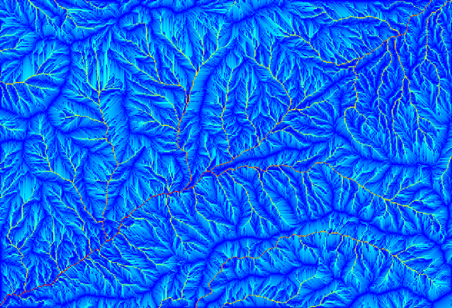
4. The catchment area (also known as flow accumulation) can be used to set a threshold for channel initiation. This can be done using the Channel network algorithm.

   • Initiation grid: use the catchment area layer and not the logarithm one.

   • Initiation threshold: 10.000.000

   • Initiation type: Greater than

   

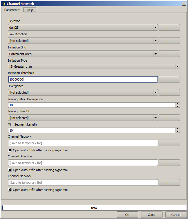
   If you increase the Initiation threshold value, you will get a more sparse channel network. If you decrease it, you will get a denser one. With the proposed value, this is what you get.

   

   The image above shows just the resulting vector layer and the DEM, but there should be also a raster layer with the same channel network. That raster will be, in fact, the layer we will be using.

5. Now, we will use the Watersheds basins algorithm to delineate the subbasins corresponding to that channel network, using as outlet points all the junctions in it. Here is how you have to set the corresponding parameters dialog.

   

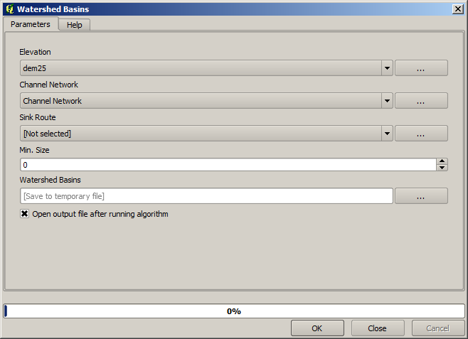
   다음이 그 결과입니다.

   

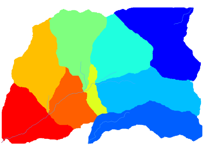
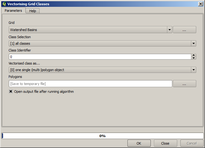
6. This is a raster result. You can vectorise it using the Vectorising grid classes algorithm.

   

   

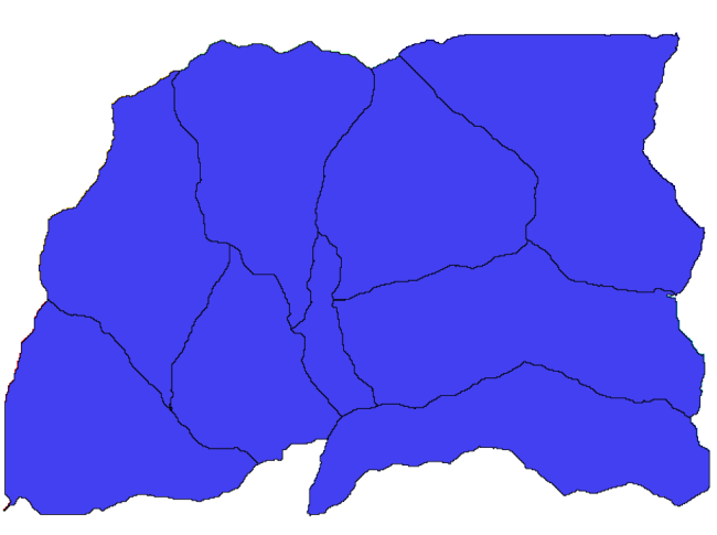
이제 이 소분지들 가운데 하나가 담고 있는 표고 값들에 대한 통계를 계산해봅시다. 해당 소분지 안의 표고만을 나타내는 레이어를 생성한 다음 해당 통계를 계산하는 알고리듬에 넘겨주면 됩니다.

1. First, let’s clip the original DEM with the polygon representing a subbasin. We will use the Clip raster with polygon algorithm. If we select a single subbasin polygon and then call the clipping algorithm, we can clip the DEM to the area covered by that polygon, since the algorithm is aware of the selection.

   1. Select a polygon

      

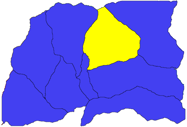
   2. Call the clipping algorithm with the following parameters:

      

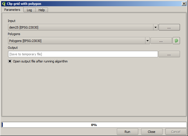
      The element selected in the input field is, of course, the DEM we want to clip.

      다음과 같은 결과를 얻게 됩니다.

      

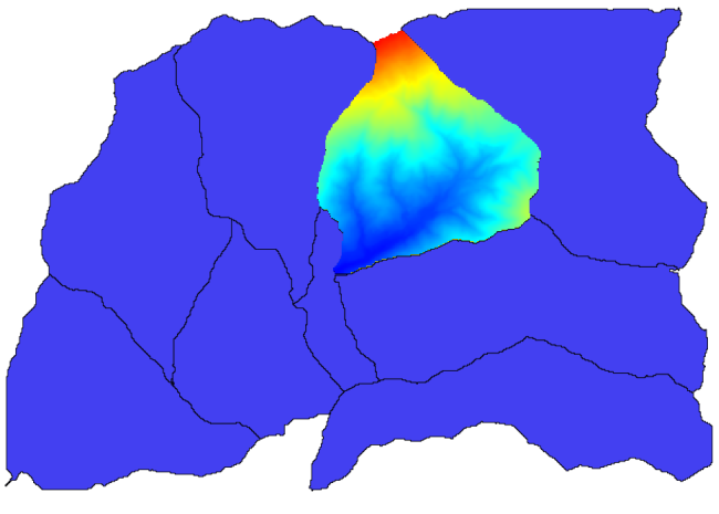
2. This layer is ready to be used in the Raster layer statistics algorithm.

   

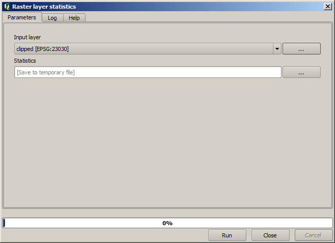
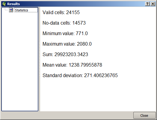
   다음과 같은 통계를 산출할 것입니다.

   

다른 강의에서도 분지 계산 과정 및 통계 계산을 – 다른 요소들이 어떻게 이 두 계산을 자동화해서 좀 더 효율적으로 작업할 수 있는지 알아보기 위해 – 모두 사용할 것입니다.