중요
번역은 여러분이 참여할 수 있는 커뮤니티 활동입니다. 이 페이지는 현재 92.86% 번역되었습니다.
17.16. 수문학적 분석
참고
이 수업에서는 수문학적 분석을 수행할 것입니다. 이 분석은 분석 워크플로에 대한 매우 훌륭한 예이기 때문에, 이어지는 수업들에서도 사용될 것입니다. 이 분석을 통해 몇몇 고급 기능들도 소개하겠습니다.
이 수업의 목표: DEM으로부터 수로망(channel network)을 추출하고, 유역(watershed)의 윤곽을 그리고, 몇몇 통계를 계산하기.
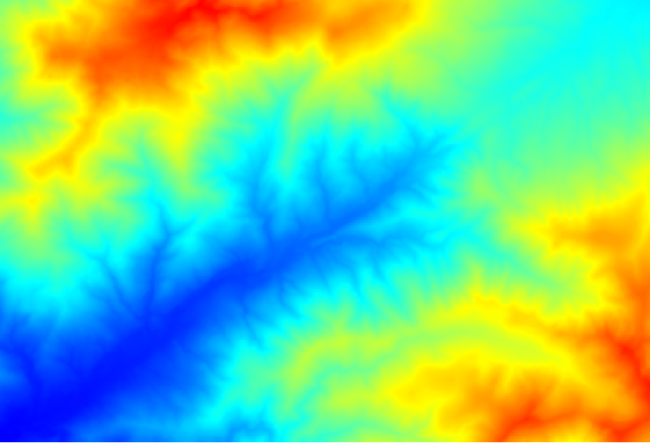
먼저 이 수업에 해당하는 프로젝트를 불러오십시오. DEM 하나만을 담고 있습니다.
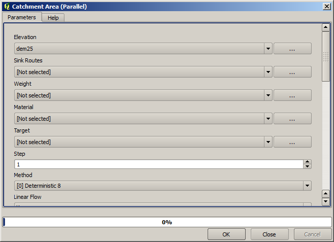
The first module to execute is Catchment area (in some SAGA versions it is called Flow accumulation (Top Down)). You can use any of the others named Catchment area. They have different algorithms underneath, but the results are basically the same.
Elevation 필드에 DEM을 선택하고, 나머지 파라미터들은 기본값대로 두십시오.
Some algorithms calculate many layers, but the Catchment Area layer is the only one we will be using. You can get rid of the other ones if you want.
이 레이어의 렌더링에서는 그렇게 많은 정보를 알 수가 없습니다.
그 이유를 알려면 히스토그램을 살펴보면 됩니다. 값들이 균등하게 분포되어 있지 않다는 사실을 알 수 있을 겁니다. (아주 높은 값을 가진 셀들이 몇 개 있습니다. 바로 수로망에 해당하는 셀들입니다.) Raster calculator 알고리즘을 사용해서 집수 지역 값의 로그를 계산하면 훨씬 많은 정보를 가진 레이어를 얻게 될 것입니다.
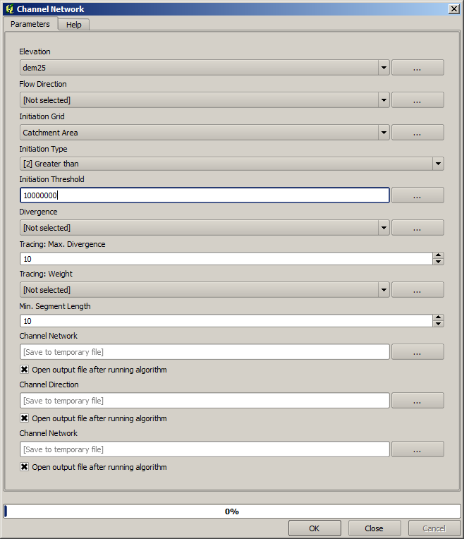
(흐름 누적이라고도 하는) 집수 지역을 사용해서 수로 시작(channel initiation)의 임계값을 설정할 수 있습니다. Channel network 알고리즘을 사용하면 됩니다.
Initiation grid: 로그 값 레이어 말고 집수 지역 레이어를 사용하십시오.
Initiation threshold:
10.000.000Initiation type: 초과(Greater than)
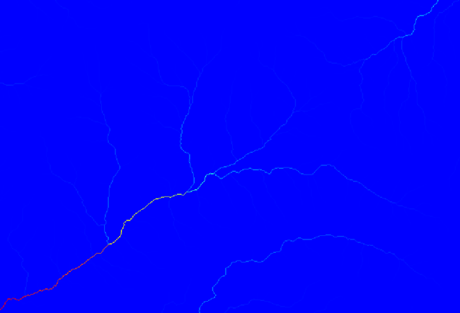
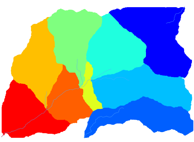
Initiation threshold 값을 증가시키면 더 성긴 수로망을 얻게 될 것입니다. 값을 감소시키면 더 빽빽한 수로망을 얻게 될 것입니다. 앞에서 제안한 값을 사용하는 경우 다음을 얻을 것입니다.

이 이미지는 생성된 벡터 레이어와 DEM만 보여주지만, 동일한 수로망을 가진 래스터 레이어도 있어야 할 것입니다. 사실 그 래스터 레이어를 사용하게 될 테니까요.
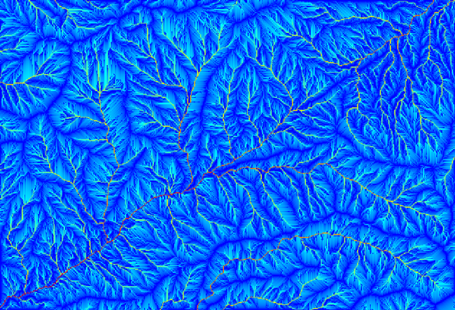
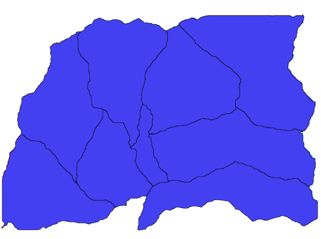
이제 Watersheds basins 알고리즘을 통해, 수로망 안에 있는 모든 연결 지점(junction)을 유출점(outlet point)으로 사용해서 이 수로망에 해당하는 소분지(subbasin)들의 윤곽을 그릴 겁니다.

다음이 그 결과입니다.
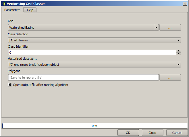
이 레이어는 래스터 레이어입니다. Vectorising grid classes 알고리즘을 사용해서 벡터화할 수 있습니다.
이제 이 소분지들 가운데 하나가 담고 있는 표고값들에 대한 통계를 계산해봅시다. 해당 소분지 안의 표고만을 나타내는 레이어를 생성한 다음 해당 통계를 계산하는 알고리즘에 넘겨주면 됩니다.
먼저 원본 DEM을 소분지 하나를 표현하는 폴리곤으로 잘라내봅시다. Clip raster with polygon 알고리즘을 사용할 것입니다. 소분지 폴리곤 하나를 선택한 다음 잘라내기 알고리즘을 호출하면 DEM에서 해당 폴리곤이 커버하는 영역을 잘라낼 수 있습니다. 이 알고리즘은 선택 집합을 인지하기 때문이죠.
폴리곤을 선택하십시오.
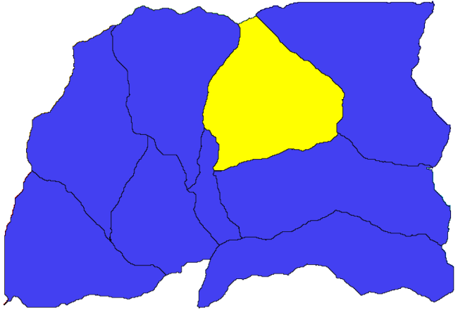
잘라내기 알고리즘을 다음 파라미터들을 사용해서 호출하십시오:

입력물 항목에 선택하는 요소는 물론 잘라내고자 하는 DEM입니다.
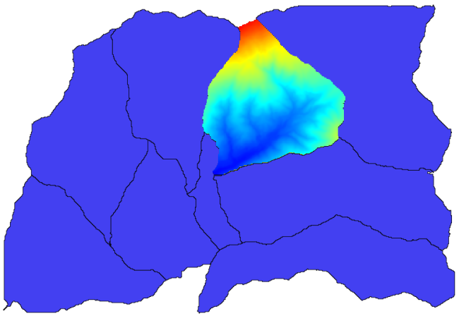
다음과 같은 결과를 얻게 됩니다.
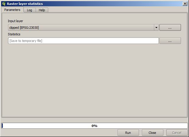
Raster layer statistics 알고리즘에 이 레이어를 사용하면 됩니다.
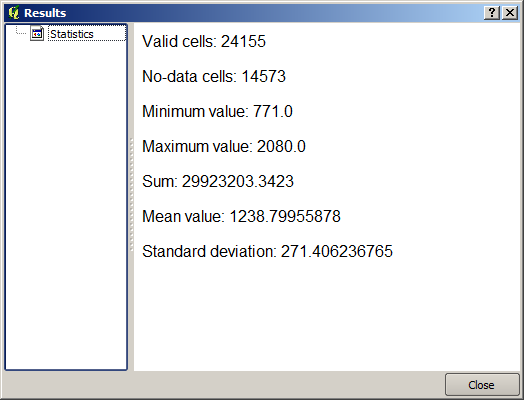
다음과 같은 통계를 산출할 것입니다.
다른 수업에서도 분지 계산 과정 및 통계 계산을 — 다른 요소들이 어떻게 이 두 계산을 자동화해서 좀 더 효율적으로 작업할 수 있는지 알아보기 위해 — 모두 사용할 것입니다.