17.23. Mais interpolação
Nota
Este capítulo mostra outro caso onde algoritmos de interpolação são usados.
Interpolation is a common technique, and it can be used to demonstrate several techniques that can be applied using the QGIS processing framework. This lesson uses some interpolation algorithms that were already introduced, but has a different approach.
Os dados para esta lição contém também uma camada de pontos, neste caso com dados de elevação. Nós estamos indo para interpolar-se muito da mesma maneira como fizemos na lição anterior, mas desta vez, vamos salvar parte dos dados originais para usá-lo para avaliar a qualidade do processo de interpolação.
First, we have to rasterize the points layer and fill the resulting no–data cells, but using just a fraction of the points in the layer. We will save 10% of the points for a later check, so we need to have 90% of the points ready for the interpolation. To do so, we could use the Split shapes layer randomly algorithm, which we have already used in a previous lesson, but there is a better way to do that, without having to create any new intermediate layer. Instead of that, we can just select the points we want to use for the interpolation (the 90% fraction), and then run the algorithm. As we have already seen, the rasterizing algorithm will use only those selected points and ignore the rest. The selection can be done using the Random selection algorithm. Run it with the following parameters.
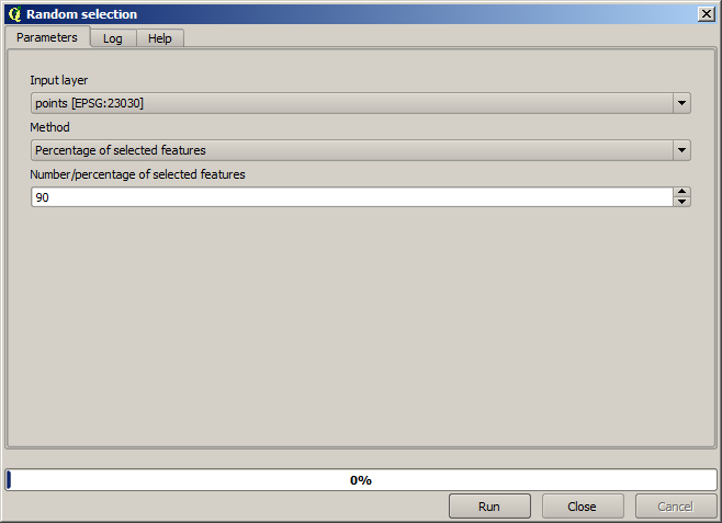
That will select 90% of the points in the layer to rasterize
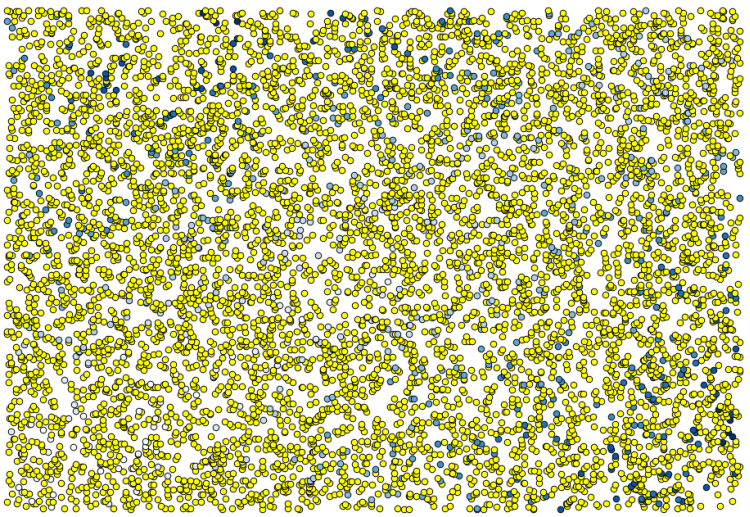
A seleção é aleatória, portanto, sua seleção pode ser diferente da seleção mostrada na imagem acima.
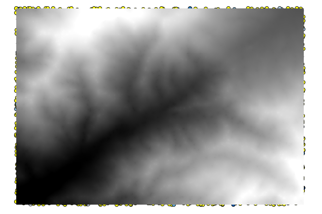
Now run the Rasterize algorithm to get the first raster layer, and then run the Close gaps algorithm to fill the no–data cells [Cell resolution: 100 m].
Para checar a qualidade da interpolação, nós agora podemos usar os pontos que não estão selecionados. Neste ponto, nós sabemos a elevação real (o valor na camada de pontos) e a elevação de interpolação (o valor na camada raster interpolada). Podemos comparar as duas, computando as diferenças entre os valores.
Como iremos usar os pontos que não estão selecionados, vamos inverter a seleção.
Os pontos contêm os valores originais, mas não os interpolados. Para adicioná-los em um novo campo, podemos usar o algoritmo Adicionar valores raster aos pontos
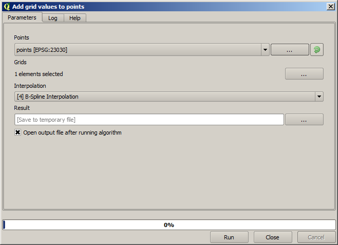
The raster layer to select (the algorithm supports multiple raster, but we just need one) is the resulting one from the interpolation. We have renamed it to interpolate and that layer name is the one that will be used for the name of the field to add.
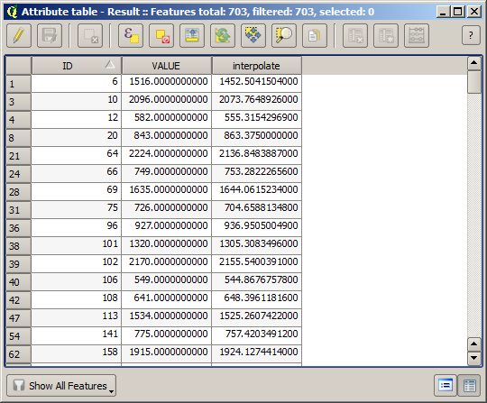
Agora temos uma camada vetorial que contém ambos valores, com pontos que não foram usados para a interpolação.
Agora, usaremos a calculadora de campo para esta tarefa. Abra o algoritmo Calculadora de campo e execute-a com os seguintes parâmetros.
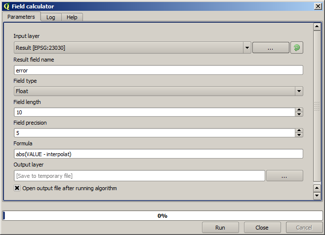
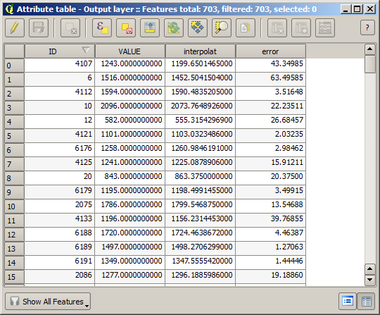
If your field with the values from the raster layer has a different name, you should modify the above formula accordingly. Running this algorithm, you will get a new layer with just the points that we haven’t used for the interpolation, each of them containing the difference between the two elevation values.
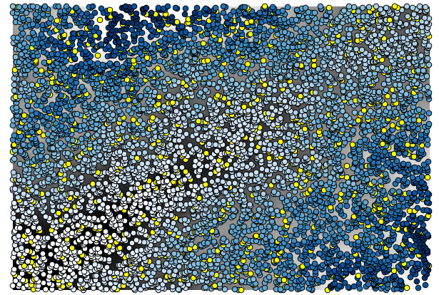
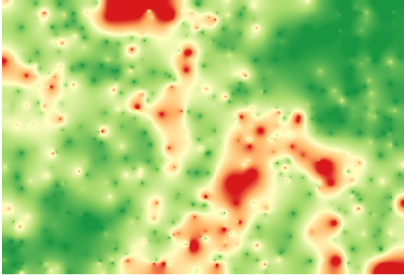
Representar essa camada de acordo com esse valor nos dará uma primeira idéia de onde as maiores discrepâncias são encontradas.
Interpolating that layer will get you a raster layer with the estimated error in all points of the interpolated area.
You can also get the same information (difference between original point values and interpolated ones) directly with .
Seus resultados podem ser diferentes desses, pois há um componente aleatório introduzido ao executar a seleção aleatória, no início desta lição.