17.23. More interpolation
Примечание
This chapter shows another practical case where interpolation algorithms are used.
Interpolation is a common technique, and it can be used to demonstrate several techniques that can be applied using the QGIS processing framework. This lesson uses some interpolation algorithms that were already introduced, but has a different approach.
The data for this lesson contains also a points layer, in this case with elevation data. We are going to interpolate it much in the same way as we did in the previous lesson, but this time we will save part of the original data to use it for assessing the quality of the interpolation process.
First, we have to rasterize the points layer and fill the resulting no–data cells, but using just a fraction of the points in the layer. We will save 10% of the points for a later check, so we need to have 90% of the points ready for the interpolation. To do so, we could use the Split shapes layer randomly algorithm, which we have already used in a previous lesson, but there is a better way to do that, without having to create any new intermediate layer. Instead of that, we can just select the points we want to use for the interpolation (the 90% fraction), and then run the algorithm. As we have already seen, the rasterizing algorithm will use only those selected points and ignore the rest. The selection can be done using the Random selection algorithm. Run it with the following parameters.
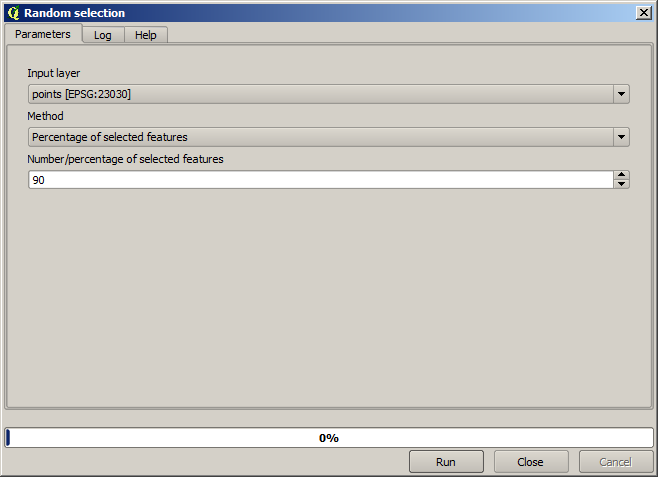
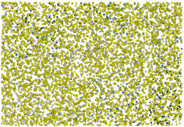
That will select 90% of the points in the layer to rasterize
The selection is random, so your selection might differ from the selection shown in the above image.
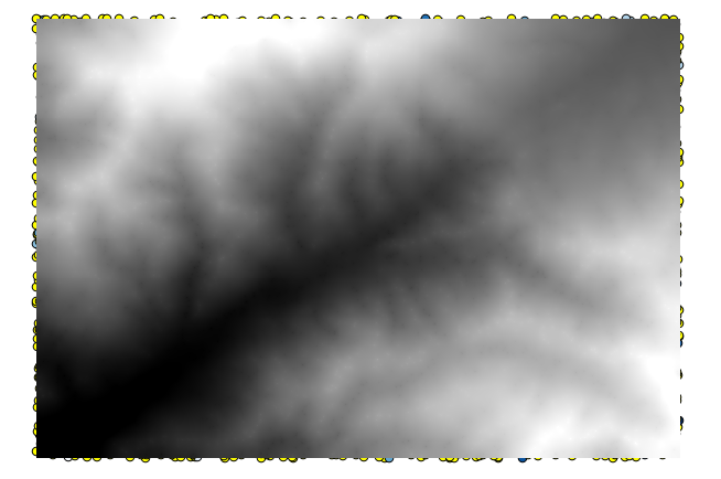
Now run the Rasterize algorithm to get the first raster layer, and then run the Close gaps algorithm to fill the no–data cells [Cell resolution: 100 m].
To check the quality of the interpolation, we can now use the points that are not selected. At this point, we know the real elevation (the value in the points layer) and the interpolated elevation (the value in the interpolated raster layer). We can compare the two by computing the differences between those values.
Since we are going to use the points that are not selected, first, let’s invert the selection.
The points contain the original values, but not the interpolated ones. To add them in a new field, we can use the Add raster values to points algorithm
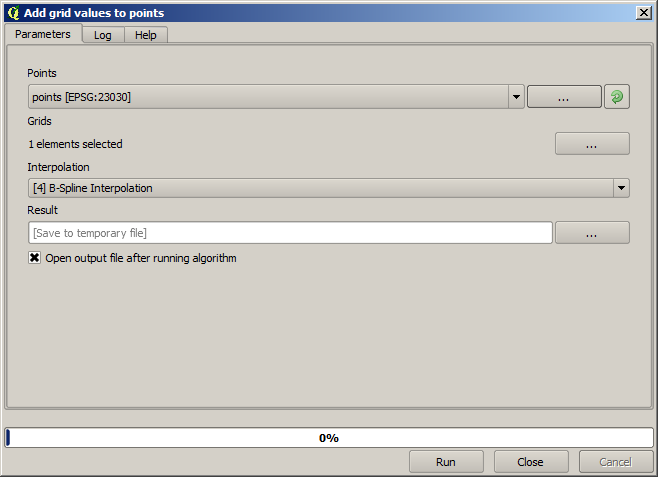
The raster layer to select (the algorithm supports multiple raster, but we just need one) is the resulting one from the interpolation. We have renamed it to interpolate and that layer name is the one that will be used for the name of the field to add.
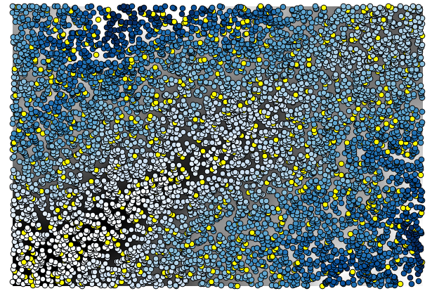
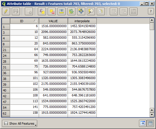
Now we have a vector layer that contains both values, with points that were not used for the interpolation.
Now, we will use the fields calculator for this task. Open the Field calculator algorithm and run it with the following parameters.
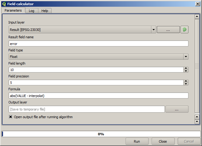
If your field with the values from the raster layer has a different name, you should modify the above formula accordingly. Running this algorithm, you will get a new layer with just the points that we haven’t used for the interpolation, each of them containing the difference between the two elevation values.
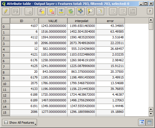
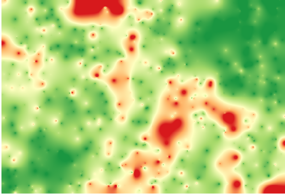
Representing that layer according to that value will give us a first idea of where the largest discrepancies are found.
Interpolating that layer will get you a raster layer with the estimated error in all points of the interpolated area.
You can also get the same information (difference between original point values and interpolated ones) directly with .
Your results might differ from these ones, since there is a random component introduced when running the random selection, at the beginning of this lesson.