5. Noțiuni de bază
This chapter provides a quick overview of installing QGIS, downloading QGIS sample data, and running a first simple session visualizing raster and vector data.
5.1. Installing QGIS
QGIS project provides different ways to install QGIS depending on your platform.
5.1.1. Installing from binaries
Standard installers are available for  MS Windows and
  macOS. Binary
packages (rpm and deb) or software repositories are provided for many flavors of
GNU/Linux
macOS. Binary
packages (rpm and deb) or software repositories are provided for many flavors of
GNU/Linux  .
.
For more information and instructions for your operating system check https://download.qgis.org.
5.1.2. Installing from source
If you need to build QGIS from source, please refer to the installation
instructions. They are distributed with the QGIS source code in a file
called INSTALL. You can also find them online at https://github.com/qgis/QGIS/blob/release-3_22/INSTALL.md.
If you want to build a particular release and not the version in development,
you should replace master with the release branch (commonly in the
release-X_Y form) in the above-mentioned link (installation instructions may differ).
5.1.3. Installing on external media
It is possible to install QGIS (with all plugins and settings) on a flash drive. This is achieved by defining a –profiles-path option that overrides the default user profile path and forces QSettings to use this directory, too. See section System Settings for additional information.
5.1.4. Downloading sample data
This user guide contains examples based on the QGIS sample dataset (also called
the Alaska dataset). Download the sample data from
https://github.com/qgis/QGIS-Sample-Data/archive/master.zip and unzip the archive
on any convenient location on your system.
Setul de date Alaska cuprinde toate datele GIS care stau la baza exemplelor și a capturilor de ecran din ghidul utilizatorului. Este inclusă, de asemenea, o mică bază de date GRASS. Proiecția datelor eșantion pentru setul de date QGIS este Alaska Albers cu Suprafețe Egale, unitățile de măsura fiind picioarele. Codul EPSG este 2964.
PROJCS["Albers Equal Area",
GEOGCS["NAD27",
DATUM["North_American_Datum_1927",
SPHEROID["Clarke 1866",6378206.4,294.978698213898,
AUTHORITY["EPSG","7008"]],
TOWGS84[-3,142,183,0,0,0,0],
AUTHORITY["EPSG","6267"]],
PRIMEM["Greenwich",0,
AUTHORITY["EPSG","8901"]],
UNIT["degree",0.0174532925199433,
AUTHORITY["EPSG","9108"]],
AUTHORITY["EPSG","4267"]],
PROJECTION["Albers_Conic_Equal_Area"],
PARAMETER["standard_parallel_1",55],
PARAMETER["standard_parallel_2",65],
PARAMETER["latitude_of_center",50],
PARAMETER["longitude_of_center",-154],
PARAMETER["false_easting",0],
PARAMETER["false_northing",0],
UNIT["us_survey_feet",0.3048006096012192]]
If you intend to use QGIS as a graphical front end for GRASS, you can find a selection of sample locations (e.g., Spearfish or South Dakota) at the official GRASS GIS website, https://grass.osgeo.org/download/data/.
5.2. Starting and stopping QGIS
QGIS can be started like any other application on your computer. This means that you can launch QGIS by:
using
the Applications menu, the Start menu, or the Dockdublu clic pe pictograma din folderul Aplicațiilor sau pe o scurtătură de pe ecran.
double clicking an existing QGIS project file (with
.qgzor.qgsextension). Note that this will also open the project.typing
qgisin a command prompt (assuming that QGIS is added to your PATH or you are in its installation folder)
To stop QGIS, use:
- opțiunea meniului , sau folosiți combinația de taste Ctrl+Q.
- , sau folosiți combinația de taste Cmd+Q.
or use the red cross at the top-right corner of the main interface of the application.
5.3. Sample Session: Loading raster and vector layers
Now that you have QGIS installed and a sample dataset available, we will demonstrate a first sample session. In this example, we will visualize a raster and a vector layer. We will use:
the
landcoverraster layer (qgis_sample_data/raster/landcover.img)and the
lakesvector layer (qgis_sample_data/gml/lakes.gml)
Where qgis_sample_data represents the path to the unzipped dataset.
Start QGIS as seen in Starting and stopping QGIS.
To load the files in QGIS:
Click on the
 Open Data Source Manager icon.
The Data Source Manager should open in Browser mode.
Open Data Source Manager icon.
The Data Source Manager should open in Browser mode.Browse to the folder
qgis_sample_data/raster/Select the ERDAS IMG file
landcover.imgand double-click it. The landcover layer is added in the background while the Data Source Manager window remains open.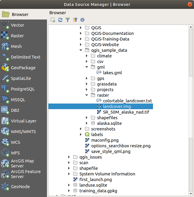
Fig. 5.1 Adding data to a new project in QGIS
To load the lakes data, browse to the folder
qgis_sample_data/gml/, and double-click thelakes.gmlfile to open it.A Coordinate Reference System Selector dialog opens. In the Filter menu, type
2964, filtering the list of Coordinate Reference Systems below.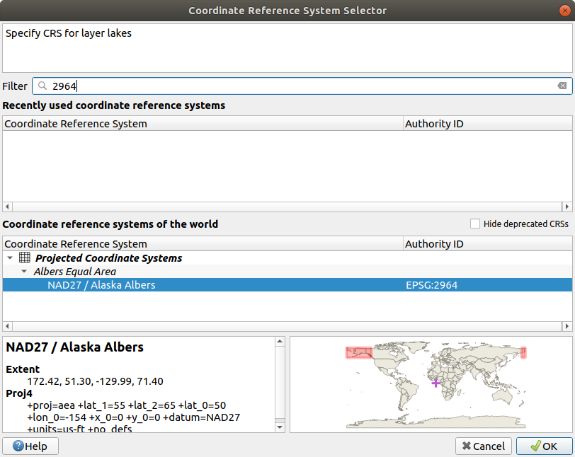
Fig. 5.2 Select the Coordinate Reference System of data
Select the NAD27 / Alaska Albers entry
Clic pe OK
Close the Data Source Manager window
You now have the two layers available in your project in some random colours. Let’s do some customization on the lakes layer.
Select the
 Zoom In tool on the Navigation toolbar
Zoom to an area with some lakes
Double-click the
lakeslayer in the map legend to open the Properties dialogTo change the lakes color:
Click on the
 Symbology tab
Select blue as fill color.
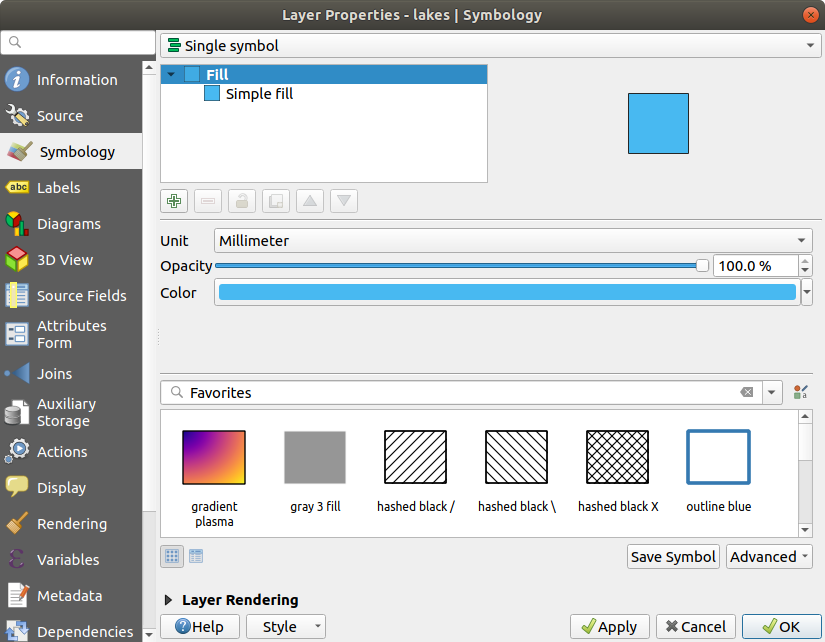
Fig. 5.3 Selecting Lakes color
Press OK. Lakes are now displayed in blue in the map canvas.
To display the name of the lakes:
Reopen the
lakeslayer Properties dialogClick on the
 Labels tab
Select Single labels in the drop-down menu to enable labeling.
From the Label with list, choose the
NAMESfield.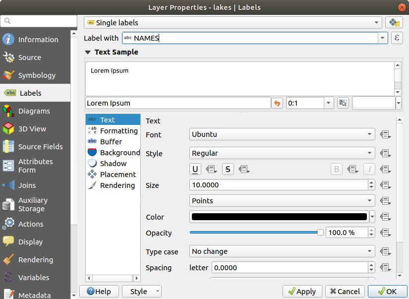
Fig. 5.4 Showing Lakes names
Press Apply. Names will now load over the boundaries.
You can improve readability of the labels by adding a white buffer around them:
Click the Buffer tab in the list on the left
Check
 Draw text buffer
Choose
3as buffer sizeClick Apply
Check if the result looks good, and update the value if needed.
Finally click OK to close the Layer Properties dialog and apply the changes.
Let’s now add some decorations in order to shape the map and export it out of QGIS:
Select menu
In the dialog that opens, check
Enable Scale Bar optionCustomize the options of the dialog as you want
Press Apply
Likewise, from the decorations menu, add more items (north arrow, copyright…) to the map canvas with custom properties.
Click

Press Save in the opened dialog
Select a file location, a format and confirm by pressing Save again.
Press
 to
store your changes as a
to
store your changes as a .qgzproject file.
That’s it! You can see how easy it is to visualize raster and vector layers in QGIS, configure them and generate your map in an image format you can use in other softwares. Let’s move on to learn more about the available functionality, features and settings, and how to use them.
Notă
To continue learning QGIS through step-by-step exercises, follow the Training manual.