23. Integrarea GRASS GIS
GRASS integration provides access to GRASS GIS databases and functionalities (see GRASS-PROJECT in Literatură și Referințe Web). The integration consists of two parts: provider and plugin. The provider allows to browse, manage and visualize GRASS raster and vector layers. The plugin can be used to create new GRASS locations and mapsets, change GRASS region, create and edit vector layers and analyze GRASS 2-D and 3-D data with more than 400 GRASS modules. In this section, we’ll introduce the provider and plugin functionalities and give some examples of managing and working with GRASS data.
The provider supports GRASS version 6 and 7, the plugin supports GRASS 6 and 7 (starting from QGIS 2.12). QGIS distribution may contain provider/plugin for either GRASS 6 or GRASS 7 or for both versions at the same time (binaries have different file names). Only one version of the provider/plugin may be loaded on runtime however.
23.1. Setul de date demonstrative
As an example, we will use the QGIS Alaska dataset (see section Downloading sample data).
It includes a small sample GRASS LOCATION with three vector layers and one
raster elevation map. Create a new folder called grassdata, download
the QGIS «Alaska» dataset qgis_sample_data.zip from
https://qgis.org/downloads/data/ and unzip the file into grassdata.
More sample GRASS LOCATIONs are available at the GRASS website at
https://grass.osgeo.org/download/data/.
23.2. Încărcarea straturilor raster și vectoriale GRASS
If the provider is loaded in QGIS, the location item with GRASS  icon is added in the browser tree under each folder item which contains GRASS location.
Go to the folder
icon is added in the browser tree under each folder item which contains GRASS location.
Go to the folder grassdata and expand location alaska and
mapset demo.
You can load GRASS raster and vector layers like any other layer from the browser either by double click on layer item or by dragging and dropping to map canvas or legend.
Sfat
Încărcarea Datelor GRASS
If you don’t see GRASS location item, verify in if GRASS vector provider is loaded.
23.3. Importing data into a GRASS LOCATION via drag and drop
This section gives an example of how to import raster and vector data into a GRASS mapset.
In QGIS browser navigate to the mapset you want to import data into.
In QGIS browser find a layer you want to import to GRASS, note that you can open another instance of the browser (Browser Panel (2)) if source data are too far from the mapset in the tree.
Drag a layer and drop it on the target mapset. The import may take some time for larger layers, you will see animated icon
 in front of new layer item
until the import finishes.
in front of new layer item
until the import finishes.
When raster data are in different CRS, they can be reprojected using an Approximate
(fast) or Exact (precise) transformation. If a link to the source raster
is created (using r.external), the source data are in the same CRS and the format
is known to GDAL, the source data CRS will be used. You can set these options in the
Browser tab in Opțiuni GRASS.
If a source raster has more bands, a new GRASS map is created for each layer with
.<band number> suffix and group of all maps with  icon is created.
External rasters have a different icon
icon is created.
External rasters have a different icon  .
.
23.4. Managing GRASS data in QGIS Browser
Copying maps: GRASS maps may be copied between mapsets within the same location using drag and drop.
Deleting maps: Right click on a GRASS map and select Delete from context menu.
Renaming maps: Right click on a GRASS map and select Rename from context menu.
23.5. Opțiuni GRASS
GRASS options may be set in GRASS Options dialog, which can be opened by right clicking on the location or mapset item in the browser and then choosing GRASS Options.
23.6. Startarea plugin-ului GRASS
To use GRASS functionalities in QGIS, you must select and load the GRASS plugin using the
Plugin Manager. To do this, go to the menu  , select
  GRASS and click
OK.
GRASS and click
OK.
The following main features are provided with the GRASS menu () when you start the GRASS plugin:
 Open Mapset
 New Mapset
 Închidere set de hărți
 Deschidere Instrumente GRASS
 Afișarea regiunii curente GRASS
 Opțiuni GRASS
23.7. Deschiderea Setului de hărți GRASS
A GRASS mapset must be opened to get access to GRASS Tools in the plugin (the tools are disabled if no mapset is open). You can open a mapset from the browser: right click on mapset item and then choose Open mapset from context menu.
23.8. GRASS LOCATION și MAPSET
Datele GRASS sunt stocate într-un director de tip GISDBASE. Acest director, denumit adesea grassdata, trebuie să existe înainte de a începe lucrul cu plugin-ul GRASS din QGIS. În interiorul acestui director, datele GRASS GIS sunt organizate în proiecte stocate, la rândul lor, în subdirectoare denumite LOCATIONs. Fiecare LOCATION este definită prin sistemul de coordonate, proiecția hărții și limitele geografice. Fiecare LOCATION poate avea mai multe MAPSETs (subdirectoare ale LOCATION) care sunt utilizate pentru a subdiviza un proiect în diferite teme sau subregiuni, ori în spații de lucru pentru membrii individuali ai unei echipe (v. Neteler & Mitasova 2008 în Literatură și Referințe Web). Pentru a analiza straturile vectoriale și raster cu ajutorul modulelor GRASS, trebuie să le importați într-o LOCATION GRASS. (Acest lucru nu este complet adevărat - cu ajutorul modulelor GRASS r.external și v.external puteți crea numai link-uri read-only către seturile de date GDAL/OGR externe acceptate, fără să fie necesar importul lor. Însă, deoarece acesta nu este modul obișnuit pentru începători de a lucra cu GRASS, această opțiune nu va fi descrisă aici.)
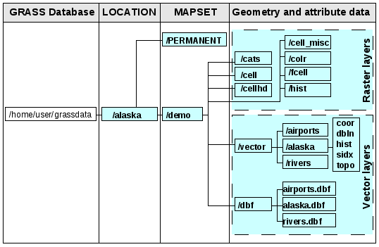
Fig. 23.1 Datele GRASS din LOCAȚIA alaska
23.9. Importați datele într-o LOCAȚIE GRASS
See section Importing data into a GRASS LOCATION via drag and drop to find how data can be easily imported by dragging and dropping in the browser.
This section gives an example of how to import raster and vector data into the
«alaska» GRASS LOCATION provided by the QGIS «Alaska» dataset in traditional
way, using standard GRASS modules.
Therefore, we use the landcover raster map landcover.img and the vector GML
file lakes.gml from the QGIS «Alaska» dataset (see Downloading sample data).
Start QGIS, apoi asigurați-vă că plugin-ul GRASS este încărcat.
In the GRASS toolbar, click the
Open MAPSET icon
to bring up the MAPSET wizard.Select as GRASS database the folder
grassdatain the QGIS Alaska dataset, asLOCATION«alaska», asMAPSET«demo» and click OK.Acum faceți clic pe pictograma
Open GRASS tools. Va apărea bara de instrumente GRASS (v. secțiunea Bara de instrumente GRASS).To import the raster map
landcover.img, click the moduler.in.gdalin the Modules Tree tab. This GRASS module allows you to import GDAL-supported raster files into a GRASSLOCATION. The module dialog forr.in.gdalappears.Răsfoiți folderul
rasterdin setul de date «Alaska» din QGIS, apoi selectați fișierullandcover.img.As raster output name, define
landcover_grassand click Run. In the Output tab, you see the currently running GRASS commandr.in.gdal -o input=/path/to/landcover.img output=landcover_grass.When it says Successfully finished, click View Output. The
landcover_grassraster layer is now imported into GRASS and will be visualized in the QGIS canvas.To import the vector GML file
lakes.gml, click the modulev.in.ogrin the Modules Tree tab. This GRASS module allows you to import OGR-supported vector files into a GRASSLOCATION. The module dialog forv.in.ograppears.Răsfoiți folderul
gmldin setul de date «Alaska» din QGIS, apoi selectați fișierullakes.gmlca fișier OGR.As vector output name, define
lakes_grassand click Run. You don’t have to care about the other options in this example. In the Output tab you see the currently running GRASS commandv.in.ogr -o dsn=/path/to/lakes.gml output=lakes\_grass.When it says Succesfully finished, click View Output. The
lakes_grassvector layer is now imported into GRASS and will be visualized in the QGIS canvas.
23.9.1. Crearea unei noi LOCAȚII GRASS
Ca exemplu, este prezentat eșantionul GRASS LOCATION alaska, care este proiectat în proiecția Albers cu Suprafețe Egale și având feet ca unitate de măsură. Acest eșantion GRASS LOCATION alaska va fi folosit pentru toate exemplele și exercițiile din următoarele secțiuni legate de GRASS. Este util să descărcați setul de date pe computerul dvs, apoi să-l instalați (v. Downloading sample data).
Start QGIS, apoi asigurați-vă că plugin-ul GRASS este încărcat.
Visualize the
alaska.shpshapefile (see section Încărcarea unui strat dintr-un fișier) from the QGIS Alaska dataset (see Downloading sample data).In the GRASS toolbar, click on the
New mapset icon
to bring up the MAPSET wizard.Select an existing GRASS database (GISDBASE) folder
grassdata, or create one for the newLOCATIONusing a file manager on your computer. Then click Next.We can use this wizard to create a new
MAPSETwithin an existingLOCATION(see section Adăugarea unui nou MAPSET) or to create a newLOCATIONaltogether. Select Create new
location (see Fig. 23.2).
Create new
location (see Fig. 23.2).Enter a name for the
LOCATION– we used «alaska» – and click Next.Define the projection by clicking on the radio button
Projection to enable the projection list.We are using Albers Equal Area Alaska (feet) projection. Since we happen to know that it is represented by the EPSG ID 2964, we enter it in the search box. (Note: If you want to repeat this process for another
LOCATIONand projection and haven’t memorized the EPSG ID, click on the CRS Status icon in the lower right-hand corner of the status bar (see
section Lucrul cu Proiecții)).
CRS Status icon in the lower right-hand corner of the status bar (see
section Lucrul cu Proiecții)).În Filtrul, inserați 2964 pentru a selecta proiecția.
Clic pe Next.
To define the default region, we have to enter the
LOCATIONbounds in the north, south, east, and west directions. Here, we simply click on the button Set Current QGIS Extent, to apply the extent of the loaded layeralaska.shpas the GRASS default region extent.Clic pe Next.
We also need to define a
MAPSETwithin our newLOCATION(this is necessary when creating a newLOCATION). You can name it whatever you like - we used «demo». GRASS automatically creates a specialMAPSETcalledPERMANENT, designed to store the core data for the project, its default spatial extent and coordinate system definitions (see Neteler & Mitasova 2008 in Literatură și Referințe Web).Check out the summary to make sure it’s correct and click Finish.
Sunt create noua
LOCATION, «alaska», și douăMAPSETs, «demo» și «PERMANENT». Setul deschis în mod curent este «demo», așa cum l-ați definit.Observați că unele instrumente din bara de instrumente GRASS, dezactivate anterior, sunt acum activate.
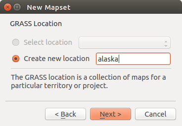
Fig. 23.2 Crearea unei LOCAȚII GRASS noi, sau a unui nou SET DE HĂRȚI în QGIS
If that seemed like a lot of steps, it’s really not all that bad and a very quick
way to create a LOCATION. The LOCATION «alaska» is now ready for
data import (see section Importați datele într-o LOCAȚIE GRASS). You can also use the already-existing
vector and raster data in the sample GRASS LOCATION «alaska»,
included in the QGIS «Alaska» dataset Downloading sample data, and move on to
section Modelul de date vectoriale GRASS.
23.9.2. Adăugarea unui nou MAPSET
A user has write access only to a GRASS MAPSET which he or she created. This
means that besides access to your own MAPSET, you can read maps in other users»
MAPSETs (and they can read yours), but you can modify or remove only the maps in
your own MAPSET.
All MAPSETs include a WIND file that stores the current boundary
coordinate values and the currently selected raster resolution (see Neteler & Mitasova
2008 in Literatură și Referințe Web, and section Regiunea instrumentelor GRASS).
Start QGIS, apoi asigurați-vă că plugin-ul GRASS este încărcat.
In the GRASS toolbar, click on the
New mapset icon
to bring up the MAPSET wizard.Selectați folderul
grassdataal bazei de date GRASS (GISDBASE) cu locațiaLOCATION«alaska», în care dorim să adăugăm un nouMAPSETdenumit «test».Clic pe Next.
We can use this wizard to create a new
MAPSETwithin an existingLOCATIONor to create a newLOCATIONaltogether. Click on the radio button Select location
(see Fig. 23.2) and click Next.Enter the name
testfor the newMAPSET. Below in the wizard, you see a list of existingMAPSETsand corresponding owners.Click Next, check out the summary to make sure it’s all correct and click Finish.
23.10. Modelul de date vectoriale GRASS
It is important to understand the GRASS vector data model prior to digitizing. In general, GRASS uses a topological vector model. This means that areas are not represented as closed polygons, but by one or more boundaries. A boundary between two adjacent areas is digitized only once, and it is shared by both areas. Boundaries must be connected and closed without gaps. An area is identified (and labelled) by the centroid of the area.
Besides boundaries and centroids, a vector map can also contain points and lines. All these geometry elements can be mixed in one vector and will be represented in different so-called «layers» inside one GRASS vector map. So in GRASS, a layer is not a vector or raster map but a level inside a vector layer. This is important to distinguish carefully. (Although it is possible to mix geometry elements, it is unusual and, even in GRASS, only used in special cases such as vector network analysis. Normally, you should prefer to store different geometry elements in different layers.)
It is possible to store several «layers» in one vector dataset. For example, fields, forests and lakes can be stored in one vector. An adjacent forest and lake can share the same boundary, but they have separate attribute tables. It is also possible to attach attributes to boundaries. An example might be the case where the boundary between a lake and a forest is a road, so it can have a different attribute table.
The «layer» of the feature is defined by the «layer» inside GRASS. «Layer» is the number which defines if there is more than one layer inside the dataset (e.g., if the geometry is forest or lake). For now, it can be only a number. In the future, GRASS will also support names as fields in the user interface.
Atributele pot fi stocate în interiorul LOCATION GRASS în format dBase sau SQLite3, sau în tabelele bazei de date externe, cum ar fi PostgreSQL, MySQL, Oracle, etc.
Atributele din tabelele bazei de date sunt legate de elementele geometrice printr-o valoare de «categorie».
«Categoria» (key, ID) este un număr întreg atașat primitivelor geometrice, fiind folosită ca legătură către o coloană cheie, din tabelul bazei de date.
Sfat
Înțelegerea modelului de date vectoriale GRASS
The best way to learn the GRASS vector model and its capabilities is to download one of the many GRASS tutorials where the vector model is described more deeply. See https://grass.osgeo.org/learn/manuals/ for more information, books and tutorials in several languages.
23.11. Crearea unui nou strat vectorial GRASS
To create a new GRASS vector layer, select one of following items from mapset context menu in the browser:
Strat Nou, de tip Punct
Strat Nou, de tip Linie
Strat Nou, de tip Poligon
and enter a name in the dialog. A new vector map will be created and layer will be added to canvas and editing started. Selecting type of the layer does not restrict geometry types which can be digitized in the vector map. In GRASS, it is possible to organize all sorts of geometry types (point, line and polygon) in one vector map. The type is only used to add the layer to the canvas, because QGIS requires a layer to have a specific type.
It is also possible to add layers to existing vector maps selecting one of the items described above from context menu of existing vector map.
In GRASS, it is possible to organize all sorts of geometry types (point, line and area) in one layer, because GRASS uses a topological vector model, so you don’t need to select the geometry type when creating a new GRASS vector. This is different from shapefile creation with QGIS, because shapefiles use the Simple Feature vector model (see section Creating new vector layers).
23.12. Digitizarea și editarea unui strat vectorial GRASS
GRASS vector layers can be digitized using the standard QGIS digitizing tools. There are however some particularities, which you should know about, due to
GRASS topological model versus QGIS simple feature
complexity of GRASS model
multiple layers in single maps
multiple geometry types in single map
geometry sharing by multiple features from multiple layers
The particularities are discussed in the following sections.
Save, discard changes, undo, redo
Atenționare
All the changes done during editing are immediately written to vector map and related attribute tables.
Changes are written after each operation, it is however, possible to do undo/redo or discard all changes when closing editing. If undo or discard changes is used, original state is rewritten in vector map and attribute tables.
There are two main reasons for this behaviour:
It is the nature of GRASS vectors coming from conviction that user wants to do what he is doing and it is better to have data saved when the work is suddenly interrupted (for example, blackout)
Necessity for effective editing of topological data is visualized information about topological correctness, such information can only be acquired from GRASS vector map if changes are written to the map.
Bara de Instrumente
The «Digitizing Toolbar» has some specific tools when a GRASS layer is edited:
Pictogramă |
Instrument |
Scop |
|---|---|---|
|
Punct Nou |
Digitizare punct nou |
|
Linie nouă |
Digitizare linie nouă |
|
Limită Nouă |
Digitize new boundary |
|
Centroid Nou |
Digitizarea unui nou centroid (etichetarea zonei existente) |
|
New Closed Boundary |
Digitize new closed boundary |


Table GRASS Digitizing: GRASS Digitizing Tools
Sfat
Digitizarea poligoanelor în GRASS
If you want to create a polygon in GRASS, you first digitize the boundary of the polygon. Then you add a centroid (label point) into the closed boundary. The reason for this is that a topological vector model links the attribute information of a polygon always to the centroid and not to the boundary.
Category
Category, often called cat, is sort of ID. The name comes from times when GRASS vectors had only singly attribute „category”. Category is used as a link between geometry and attributes. A single geometry may have multiple categories and thus represent multiple features in different layers. Currently it is possible to assign only one category per layer using QGIS editing tools. New features have automatically assigned new unique category, except boundaries. Boundaries usually only form areas and do not represent linear features, it is however possible to define attributes for a boundary later, for example in different layer.
New categories are always created only in currently being edited layer.
It is not possible to assign more categories to geometry using QGIS editing, such data are properly represented as multiple features, and individual features, even from different layers, may be deleted.
Atribute
Attributes of currently edited layer can only be modified. If the vector map contains more layers, features of other layers will have all attributes set to «<not editable (layer #)>» to warn you that such attribute is not editable. The reason is, that other layers may have and usually have different set of fields while QGIS only supports one fixed set of fields per layer.
If a geometry primitive does not have a category assigned, a new unique category is automatically assigned and new record in attribute table is created when an attribute of that geometry is changed.
Sfat
If you want to do bulk update of attributes in table, for example using «Field Calculator»
(Using the Field Calculator), and there are features without category which you don’t want
to update (typically boundaries), you can filter them out by setting «Advanced Filter» to cat is not null.
Editing style
The topological symbology is essential for effective editing of topological data. When editing starts, a specialized «GRASS Edit» renderer is set on the layer automatically and original renderer is restored when editing is closed. The style may be customized in layer properties «Style» tab. The style can also be stored in project file or in separate file as any other style. If you customize the style, do not change its name, because it is used to reset the style when editing is started again.
Sfat
Do not save project file when the layer is edited, the layer would be stored with «Edit Style» which has no meaning if layer is not edited.
The style is based on topological information which is temporarily added to attribute table as field «topo_symbol». The field is automatically removed when editing is closed.
Sfat
Do not remove «topo_symbol» field from attribute table, that would make features invisible because the renderer is based on that column.
Acroșarea
To form an area, vertices of connected boundaries must have exactly the same coordinates. This can be achieved using snapping tool only if canvas and vector map have the same CRS. Otherwise, due conversion from map coordinates to canvas and back, the coordinate may become slightly different due to representation error and CRS transformations.
Sfat
Canvasul folosește CRS-ul stratului și la momentul editării.
Limitări
Simultaneous editing of multiple layers within the same vector at the same time is not supported. This is mainly due to the impossibility of handling multiple undo stacks for a single data source.

 On Linux and macOS only one GRASS layer can be edited at time. This is
due to a bug in GRASS which does not allow to close database drivers in random order.
This is being solved with GRASS developers.
On Linux and macOS only one GRASS layer can be edited at time. This is
due to a bug in GRASS which does not allow to close database drivers in random order.
This is being solved with GRASS developers.
Sfat
Permisiuni de Editare GRASS
Trebuie să fiți proprietarul MAPSET GRASS, pentru a-l putea edita. Este imposibilă editarea datelor din straturile MAPSET care nu vă aparține, chiar dacă aveți permisiunea de scriere.
23.13. Regiunea instrumentelor GRASS
The region definition (setting a spatial working window) in GRASS is important
for working with raster layers. Vector analysis is by default not limited to any
defined region definitions. But all newly created rasters will have the spatial
extension and resolution of the currently defined GRASS region, regardless of
their original extension and resolution. The current GRASS region is stored in
the $LOCATION/$MAPSET/WIND file, and it defines north, south, east and
west bounds, number of columns and rows, horizontal and vertical spatial resolution.
It is possible to switch on and off the visualization of the GRASS region in the QGIS
canvas using the Display current GRASS region button.
The region can be modified in «Region» tab in «GRASS Tolls» dock widget. Type in the new region bounds and resolution, and click Apply. If you click on Select the extent by dragging on canvas you can select a new region interactively with your mouse on the QGIS canvas dragging a rectangle.
The GRASS module g.region provides a lot more parameters to define an
appropriate region extent and resolution for your raster analysis. You can use
these parameters with the GRASS Toolbox, described in section Bara de instrumente GRASS.
23.14. Bara de instrumente GRASS
The Open GRASS Tools box provides GRASS module functionalities
to work with data inside a selected GRASS LOCATION and MAPSET.
To use the GRASS Toolbox you need to open a LOCATION and MAPSET
that you have write permission for (usually granted, if you created the MAPSET).
This is necessary, because new raster or vector layers created during analysis
need to be written to the currently selected LOCATION and MAPSET.
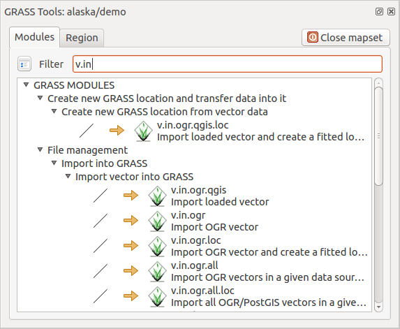
Fig. 23.3 GRASS Toolbox and Module Tree
23.14.1. Lucrul cu modulele GRASS
The GRASS shell inside the GRASS Toolbox provides access to almost all (more than 300) GRASS modules in a command line interface. To offer a more user-friendly working environment, about 200 of the available GRASS modules and functionalities are also provided by graphical dialogs within the GRASS plugin Toolbox.
A complete list of GRASS modules available in the graphical Toolbox in QGIS version 3.22 is available in the GRASS wiki at https://grasswiki.osgeo.org/wiki/GRASS-QGIS_relevant_module_list.
De asemenea, este posibilă personalizarea conținutul Instrumentarului GRASS. Această procedură este descrisă în secțiunea Personalizarea Barei de Instrumente GRASS.
As shown in Fig. 23.3, you can look for the appropriate GRASS module using the thematically grouped Modules Tree or the searchable Modules List tab.
By clicking on a graphical module icon, a new tab will be added to the Toolbox dialog, providing three new sub-tabs: Options, Output and Manual.
Opțiuni
The Options tab provides a simplified module dialog where you can usually select a raster or vector layer visualized in the QGIS canvas and enter further module-specific parameters to run the module.
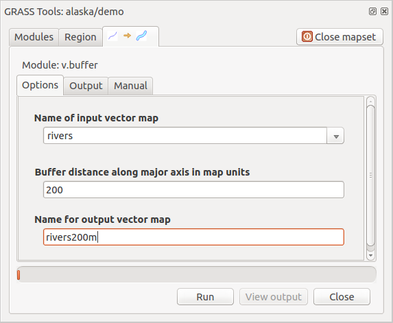
Fig. 23.4 GRASS Toolbox Module Options
The provided module parameters are often not complete to keep the dialog simple. If you want to use further module parameters and flags, you need to start the GRASS shell and run the module in the command line.
A new feature since QGIS 1.8 is the support for a Show Advanced Options
button below the simplified module dialog in the Options tab. At the
moment, it is only added to the module v.in.ascii as an example of use, but it will
probably be part of more or all modules in the GRASS Toolbox in future versions
of QGIS. This allows you to use the complete GRASS module options without the need
to switch to the GRASS shell.
Rezultat
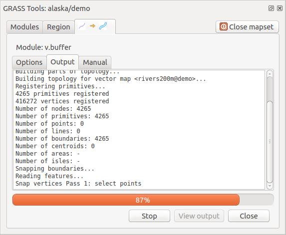
Fig. 23.5 GRASS Toolbox Module Output
The Output tab provides information about the output status of the
module. When you click the Run button, the module switches to the
Output tab and you see information about the analysis process. If
all works well, you will finally see a Successfully finished message.
Manual
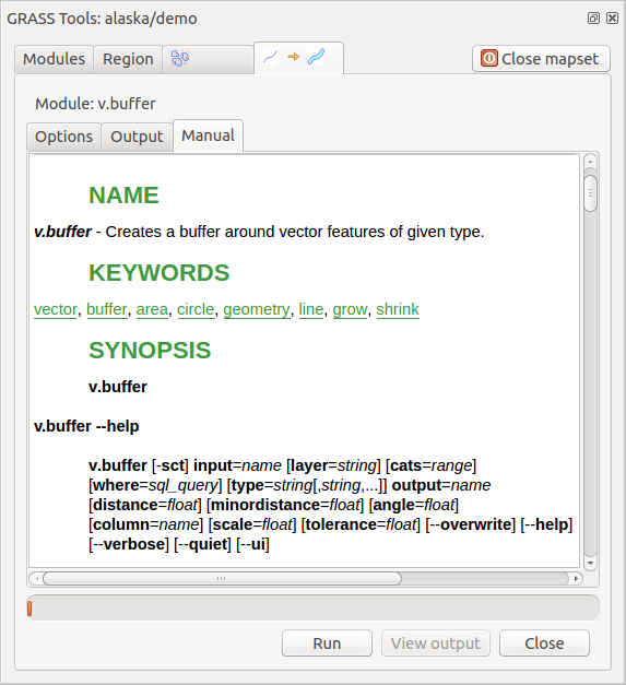
Fig. 23.6 GRASS Toolbox Module Manual
The Manual tab shows the HTML help page of the GRASS module. You can
use it to check further module parameters and flags or to get a deeper knowledge
about the purpose of the module. At the end of each module manual page, you see
further links to the Main Help index, the Thematic index and the
Full index. These links provide the same information as the
module g.manual.
Sfat
Afișează imediat rezultatele
Dacă doriți să afișați imediat rezultatele calculelor dvs în canevasul hărții, puteți folosi butonul «Vizualizare Output», din partea de jos a filei modulului.
23.14.2. Exemple de module GRASS
Următoarele exemple vor demonstra puterea unora dintre modulele GRASS.
23.14.2.1. Crearea curbelor de nivel
The first example creates a vector contour map from an elevation raster (DEM).
Here, it is assumed that you have the Alaska LOCATION set up as explained
in section Importați datele într-o LOCAȚIE GRASS.
First, open the location by clicking the
Open mapset button and choosing the Alaska location.Now open the Toolbox with the
Open GRASS tools button.În lista de de unelte pentru categorii, faceți dublu-clic pe .
Now a single click on the tool r.contour will open the tool dialog as explained above (see Lucrul cu modulele GRASS).
In the Name of input raster map enter
gtopo30.Type into the Increment between Contour levels
 the value 100. (This will create contour lines at intervals of 100 meters.)
Introduceți în Name for output vector map `numele ``ctour_100`.
Click Run to start the process. Wait for several moments until the message
Successfully finishedappears in the output window. Then click View Output and Close.
Deoarece aceasta este o regiune mare, va dura ceva timp până la afișare. După ce se termină randarea, puteți deschide fereastra cu proprietățile stratului, pentru a schimba culoarea liniei astfel încât conturul să apară clar pe rasterul de elevație, la fel ca în Dialogul Proprietăților Vectoriale.
Next, zoom in to a small, mountainous area in the center of Alaska. Zooming in close, you will notice that the contours have sharp corners. GRASS offers the v.generalize tool to slightly alter vector maps while keeping their overall shape. The tool uses several different algorithms with different purposes. Some of the algorithms (i.e., Douglas Peuker and Vertex Reduction) simplify the line by removing some of the vertices. The resulting vector will load faster. This process is useful when you have a highly detailed vector, but you are creating a very small-scale map, so the detail is unnecessary.
Sfat
Instrumentul de simplificare
Note that QGIS has a tool that works just like the GRASS v.generalize Douglas-Peuker algorithm.
However, the purpose of this example is different. The contour lines created by
r.contour have sharp angles that should be smoothed. Among the v.generalize
algorithms, there is Chaiken’s, which does just that (also Hermite splines). Be
aware that these algorithms can add additional vertices to the vector,
causing it to load even more slowly.
Open the GRASS Toolbox and double-click the categories , then click on the v.generalize module to open its options window.
Verificați dacă «ctour_100» apare ca Nume pentru vectorul de intrare.
From the list of algorithms, choose Chaiken’s. Leave all other options at their default, and scroll down to the last row to enter in the field Name for output vector map «ctour_100_smooth», and click Run.
The process takes several moments. Once
Successfully finishedappears in the output windows, click View Output and then Close.Puteți schimba culoarea vectorului pentru a-l afișa în mod clar pe fundalul raster, și pentru a contrasta față de curbele de nivel originale. Veți observa că noile curbe de nivel au colțuri mai fine decât originalul, în timp ce urmează fidel forma originală.
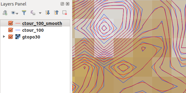
Fig. 23.7 GRASS module v.generalize to smooth a vector map
Sfat
Alte utilizări pentru r.contour
The procedure described above can be used in other equivalent situations. If you have a raster map of precipitation data, for example, then the same method will be used to create a vector map of isohyetal (constant rainfall) lines.
23.14.2.2. Crearea unui efect 3-D de umbrire
Several methods are used to display elevation layers and give a 3-D effect to maps. The use of contour lines, as shown above, is one popular method often chosen to produce topographic maps. Another way to display a 3-D effect is by hillshading. The hillshade effect is created from a DEM (elevation) raster by first calculating the slope and aspect of each cell, then simulating the sun’s position in the sky and giving a reflectance value to each cell. Thus, you get sun-facing slopes lighted; the slopes facing away from the sun (in shadow) are darkened.
Begin this example by loading the
gtopo30elevation raster. Start the GRASS Toolbox, and under the Raster category, double-click to open .Apoi faceți clic pe r.shaded.relief pentru a deschide modulul.
Change the azimuth angle
270 to 315.Enter
gtopo30_shadefor the new hillshade raster, and click Run.Când procesul se încheie, adăugați hărții rasterul reliefat. Ar trebui să-l vedeți afișat în tonuri de gri.
To view both the hillshading and the colors of the
gtopo30together, move the hillshade map below thegtopo30map in the table of contents, then open the window ofgtopo30, switch to the Transparency tab and set its transparency level to about 25%.
Ar trebui să aveți acum elevația gtopo30 cu harta de cuori și transparența setate deasupra hărții reliefului, în tonuri de gri. Pentru a observa mai bine efectele vizuale ale reliefării, desetați vizualizarea hărții gtopo30_shade, apoi resetați-o.
Folosirea consolei GRASS
The GRASS plugin in QGIS is designed for users who are new to GRASS and not familiar with all the modules and options. As such, some modules in the Toolbox do not show all the options available, and some modules do not appear at all. The GRASS shell (or console) gives the user access to those additional GRASS modules that do not appear in the Toolbox tree, and also to some additional options to the modules that are in the Toolbox with the simplest default parameters. This example demonstrates the use of an additional option in the r.shaded.relief module that was shown above.
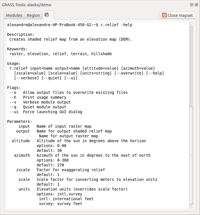
Fig. 23.8 The GRASS shell, r.shaded.relief module
The module r.shaded.relief can take a parameter zmult, which multiplies
the elevation values relative to the X-Y coordinate units so that the hillshade
effect is even more pronounced.
Load the
gtopo30elevation raster as above, then start the GRASS Toolbox and click on the GRASS shell. In the shell window, type the commandr.shaded.relief map=gtopo30 shade=gtopo30_shade2 azimuth=315 zmult=3and press Enter.After the process finishes, shift to the Browse tab and double-click on the new
gtopo30_shade2raster to display it in QGIS.As explained above, move the shaded relief raster below the
gtopo30raster in the table of contents, then check the transparency of the coloredgtopo30layer. You should see that the 3-D effect stands out more strongly compared with the first shaded relief map.
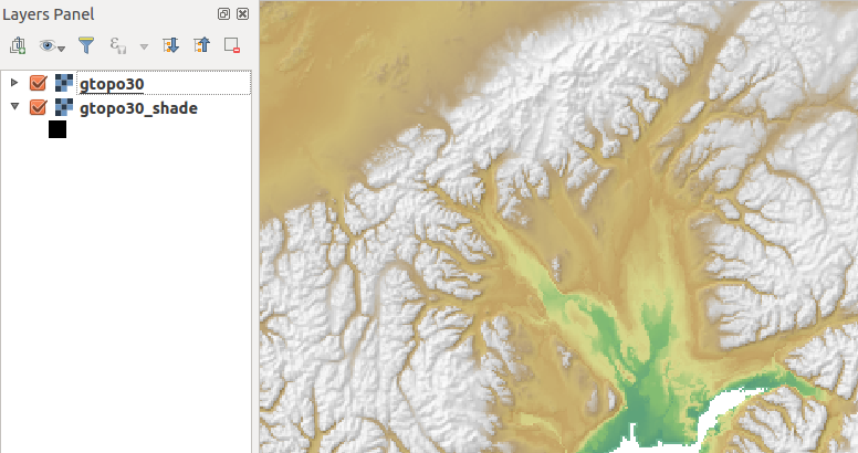
Fig. 23.9 Displaying shaded relief created with the GRASS module r.shaded.relief
23.14.2.3. Statistici raster pentru o hartă vectorială
Următorul exemplu arată modul în care un modul din GRASS poate agrega datele rastere, apoi să adauge coloanele de statistici pentru fiecare poligon din harta vectorială.
Again using the Alaska data, refer to Importați datele într-o LOCAȚIE GRASS to import the
shapefiles/trees.shpfile into GRASS.Now an intermediate step is required: centroids must be added to the imported trees map to make it a complete GRASS area vector (including both boundaries and centroids).
Din Bara de instrumente alegeți , apoi deschideți modulul v.centroids.
Introduceți «forest_areas» pentru output vector map, apoi rulați modulul.
Now load the
forest_areasvector and display the types of forests - deciduous, evergreen, mixed - in different colors: In the layer Properties window, Symbology tab, choose from Legend type «Unique value» and set the Classification field
to «VEGDESC». (Refer to the explanation of the symbology tab in
Symbology Properties of the vector section.)
«Unique value» and set the Classification field
to «VEGDESC». (Refer to the explanation of the symbology tab in
Symbology Properties of the vector section.)Mai departe, redeschideți Bara de instrumente GRASS, apoi deschideți din alte hărți.
Clic pe modulul v.rast.stats. Introduceți
gtopo30șiforest_areas.Only one additional parameter is needed: Enter column prefix
elev, and click Run. This is a computationally heavy operation, which will run for a long time (probably up to two hours).Finally, open the
forest_areasattribute table, and verify that several new columns have been added, includingelev_min,elev_max,elev_mean, etc., for each forest polygon.
23.14.3. Personalizarea Barei de Instrumente GRASS
Nearly all GRASS modules can be added to the GRASS Toolbox. An XML interface is provided to parse the pretty simple XML files that configure the modules» appearance and parameters inside the Toolbox.
Un fișier XML eșantion, pentru generarea modulului v.buffer (v.buffer.qgm) arată în felul următor:
<?xml version="1.0" encoding="UTF-8"?>
<!DOCTYPE qgisgrassmodule SYSTEM "http://mrcc.com/qgisgrassmodule.dtd">

<qgisgrassmodule label="Vector buffer" module="v.buffer">
        <option key="input" typeoption="type" layeroption="layer" />
        <option key="buffer"/>
        <option key="output" />
</qgisgrassmodule>
The parser reads this definition and creates a new tab inside the Toolbox when you select the module. A more detailed description for adding new modules, changing a module’s group, etc., can be found at https://qgis.org/en/site/getinvolved/development/addinggrasstools.html.