10. Vector Spatial Analysis (Buffers)
|
Objectives: |
Understanding the use of buffering in vector spatial analysis. |
Keywords: |
Vector, buffer zone, spatial analysis, buffer distance, dissolve boundary, outward and inward buffer, multiple buffer |
10.1. Overview
Spatial analysis uses spatial information to extract new and additional meaning from GIS data. Usually spatial analysis is carried out using a GIS Application. GIS Applications normally have spatial analysis tools for feature statistics (e.g. how many vertices make up this polyline?) or geoprocessing such as feature buffering. The types of spatial analysis that are used vary according to subject areas. People working in water management and research (hydrology) will most likely be interested in analysing terrain and modelling water as it moves across it. In wildlife management users are interested in analytical functions that deal with wildlife point locations and their relationship to the environment. In this topic we will discuss buffering as an example of a useful spatial analysis that can be carried out with vector data.
10.2. Buffering in detail
Buffering usually creates two areas: one area that is within a specified distance to selected real world features and the other area that is beyond. The area that is within the specified distance is called the buffer zone.
A buffer zone is any area that serves the purpose of keeping real world features distant from one another. Buffer zones are often set up to protect the environment, protect residential and commercial zones from industrial accidents or natural disasters, or to prevent violence. Common types of buffer zones may be greenbelts between residential and commercial areas, border zones between countries (see Fig. 10.42), noise protection zones around airports, or pollution protection zones along rivers.
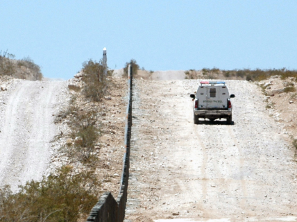
Fig. 10.42 The border between the United States of America and Mexico is separated by a buffer zone. (Photo taken by SGT Jim Greenhill 2006).
In a GIS Application, buffer zones are always represented as vector polygons enclosing other polygon, line or point features (see Fig. 10.43, Fig. 10.44, Fig. 10.45).
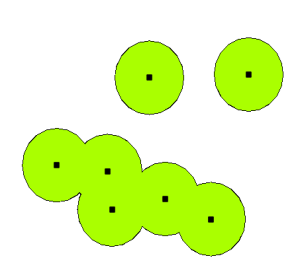
Fig. 10.43 A buffer zone around vector points.
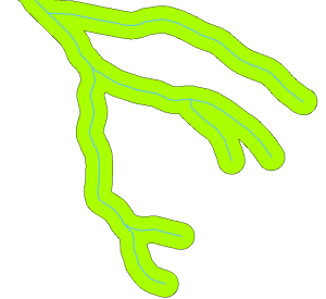
Fig. 10.44 A buffer zone around vector polylines.
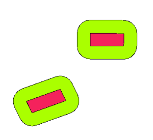
Fig. 10.45 A buffer zone around vector polygons.
10.3. Variations in buffering
There are several variations in buffering. The buffer distance or buffer size can vary according to numerical values provided in the vector layer attribute table for each feature. The numerical values have to be defined in map units according to the Coordinate Reference System (CRS) used with the data. For example, the width of a buffer zone along the banks of a river can vary depending on the intensity of the adjacent land use. For intensive cultivation the buffer distance may be bigger than for organic farming (see Figure Fig. 10.46 and Table 10.6).
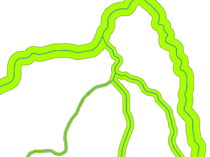
Fig. 10.46 Buffering rivers with different buffer distances.
River |
Adjacent land use |
Buffer distance (meters) |
|---|---|---|
Breede River |
Intensive vegetable cultivation |
100 |
Komati |
Intensive cotton cultivation |
150 |
Oranje |
Organic farming |
50 |
Telle river |
Organic farming |
50 |
Buffers around polyline features, such as rivers or roads, do not have to be on both sides of the lines. They can be on either the left side or the right side of the line feature. In these cases the left or right side is determined by the direction from the starting point to the end point of the line during digitising.
10.3.1. Multiple buffer zones
A feature can also have more than one buffer zone. A nuclear power plant may be buffered with distances of 10, 15, 25 and 30 km, thus forming multiple rings around the plant as part of an evacuation plan (see Fig. 10.47).
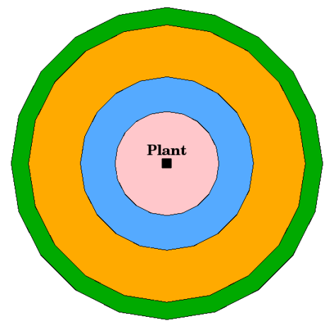
Fig. 10.47 Buffering a point feature with distances of 10, 15, 25 and 30 km.
10.3.2. Buffering with intact or dissolved boundaries
Buffer zones often have dissolved boundaries so that there are no overlapping areas between the buffer zones. In some cases though, it may also be useful for boundaries of buffer zones to remain intact, so that each buffer zone is a separate polygon and you can identify the overlapping areas (see Figure Fig. 10.48).
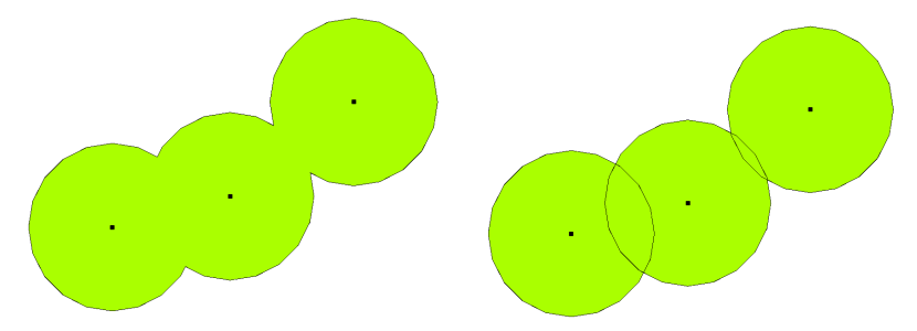
Fig. 10.48 Buffer zones with dissolved (left) and with intact boundaries (right) showing overlapping areas.
10.3.3. Buffering outward and inward
Buffer zones around polygon features are usually extended outward from a polygon boundary but it is also possible to create a buffer zone inward from a polygon boundary. Say, for example, the Department of Tourism wants to plan a new road around Robben Island and environmental laws require that the road is at least 200 meters inward from the coastline. They could use an inward buffer to find the 200 m line inland and then plan their road not to go beyond that line.
10.4. Common problems / things to be aware of
Most GIS Applications offer buffer creation as an analysis tool, but the options for creating buffers can vary. For example, not all GIS Applications allow you to buffer on either the left side or the right side of a line feature, to dissolve the boundaries of buffer zones or to buffer inward from a polygon boundary.
A buffer distance always has to be defined as a whole number (integer) or a decimal number (floating point value). This value is defined in map units (meters, feet, decimal degrees) according to the Coordinate Reference System (CRS) of the vector layer.
10.5. More spatial analysis tools
Buffering is an important and often used spatial analysis tool but there are many others that can be used in a GIS and explored by the user.
Spatial overlay is a process that allows you to identify the relationships between two polygon features that share all or part of the same area. The output vector layer is a combination of the input features information (see Fig. 10.49).
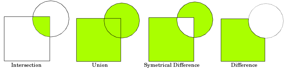
Fig. 10.49 Spatial overlay with two input vector layers (a_input = rectangle, b_input = circle). The resulting vector layer is displayed in green.
Typical spatial overlay examples are:
Intersection: The output layer contains all areas where both layers overlap (intersect).
Union: the output layer contains all areas of the two input layers combined.
Symmetrical difference: The output layer contains all areas of the input layers except those areas where the two layers overlap (intersect).
Difference: The output layer contains all areas of the first input layer that do not overlap (intersect) with the second input layer.
10.6. What have we learned?
Let’s wrap up what we covered in this worksheet:
Buffer zones describe areas around real world features.
Buffer zones are always vector polygons.
A feature can have multiple buffer zones.
The size of a buffer zone is defined by a buffer distance.
A buffer distance has to be an integer or floating point value.
A buffer distance can be different for each feature within a vector layer.
Polygons can be buffered inward or outward from the polygon boundary.
Buffer zones can be created with intact or dissolved boundaries.
Besides buffering, a GIS usually provides a variety of vector analysis tools to solve spatial tasks.
10.7. Now you try!
Here are some ideas for you to try with your learners:
Because of dramatic traffic increase, the town planners want to widen the main road and add a second lane. Create a buffer around the road to find properties that fall within the buffer zone (see Fig. 10.50).
For controlling protesting groups, the police want to establish a neutral zone to keep protesters at least 100 meters from a building. Create a buffer around a building and colour it so that event planners can see where the buffer area is.
A truck factory plans to expand. The siting criteria stipulate that a potential site must be within 1 km of a heavy-duty road. Create a buffer along a main road so that you can see where potential sites are.
Imagine that the city wants to introduce a law stipulating that no bottle stores may be within a 1000 meter buffer zone of a school or a church. Create a 1 km buffer around your school and then go and see if there would be any bottle stores too close to your school.
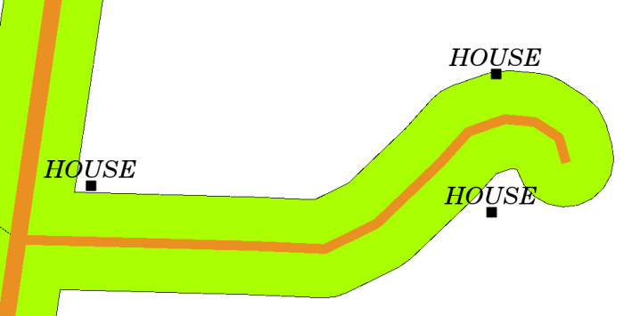
Fig. 10.50 Buffer zone (green) around a roads map (brown). You can see which houses fall within the buffer zone, so now you could contact the owner and talk to him about the situation.
10.8. Something to think about
If you don’t have a computer available, you can use a toposheet and a compass to create buffer zones around buildings. Make small pencil marks at an equal distance all along your feature using the compass, then connect the marks using a ruler!
10.9. Further reading
Books:
Galati, Stephen R. (2006). Geographic Information Systems Demystified. Artech House Inc. ISBN: 158053533X
Chang, Kang-Tsung (2006). Introduction to Geographic Information Systems. 3rd Edition. McGraw Hill. ISBN: 0070658986
DeMers, Michael N. (2005). Fundamentals of Geographic Information Systems. 3rd Edition. Wiley. ISBN: 9814126195
The QGIS User Guide also has more detailed information on analysing vector data in QGIS.
10.10. What’s next?
In the section that follows we will take a closer look at interpolation as an example of spatial analysis you can do with raster data.