17.16. Hydrologische Analyse
Bemerkung
In dieser Lektion werden wir einige hydrologische Untersuchungen durchführen. Diese werden in einigen der anderen Übungen gebraucht, da diese ein sehr gutes Beispiel für einen analytischen Workflow darstellt und diese für einige erweiterte Funktionen genutzt werden.
Objectives: Starting with a DEM, we are going to extract a channel network, delineate watersheds and calculate some statistics.
Zu Beginn müssen die Übungsdaten in das Projekt geladen werden, welche lediglich ein DGM bzw. DEM ist.

The first module to execute is Catchment area (in some SAGA versions it is called Flow accumulation (Top Down)). You can use any of the others named Catchment area. They have different algorithms underneath, but the results are basically the same.
Select the DEM in the Elevation field, and leave the default values for the rest of the parameters.
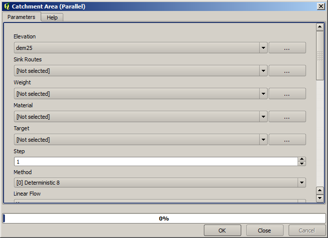
Some algorithms calculate many layers, but the Catchment Area layer is the only one we will be using. You can get rid of the other ones if you want.
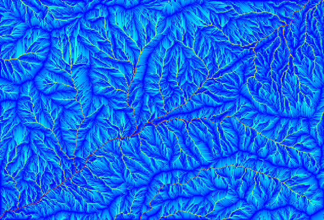
Der erstellte Layer ist nicht sonderlich Informativ.
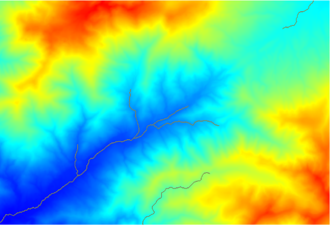
To know why, you can have a look at the histogram and you will see that values are not evenly distributed (there are a few cells with very high value, those corresponding to the channel network). Use the Raster calculator algorithm to calculate the logarithm of the catchment value area and you will get a layer with much more information
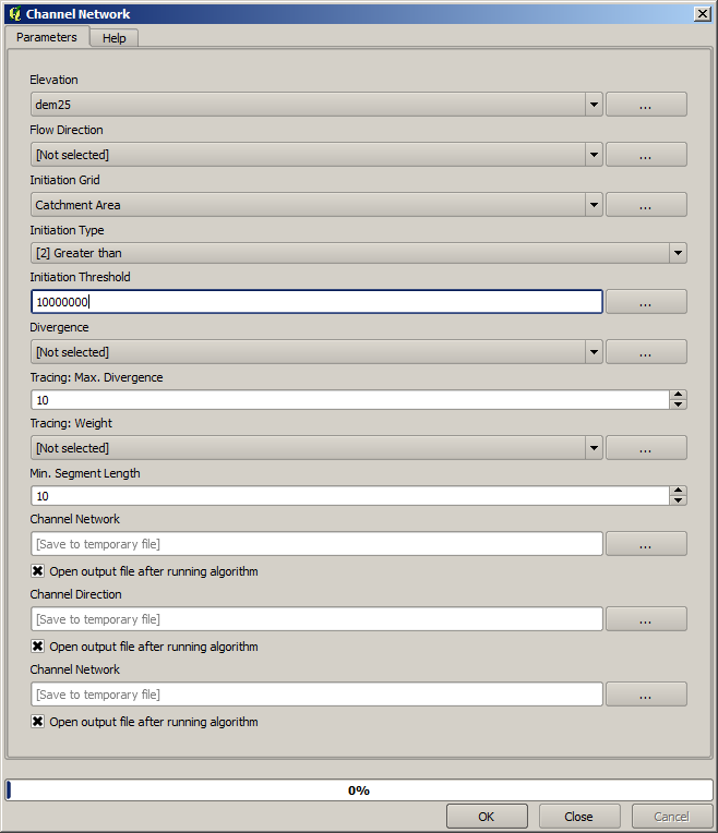
The catchment area (also known as flow accumulation) can be used to set a threshold for channel initiation. This can be done using the Channel network algorithm.
Initiation grid: use the catchment area layer and not the logarithm one.
Initiation threshold:
10.000.000Initiation type: Greater than
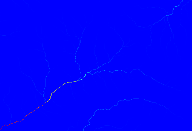
If you increase the Initiation threshold value, you will get a more sparse channel network. If you decrease it, you will get a denser one. With the proposed value, this is what you get.
The image above shows just the resulting vector layer and the DEM, but there should be also a raster layer with the same channel network. That raster will be, in fact, the layer we will be using.
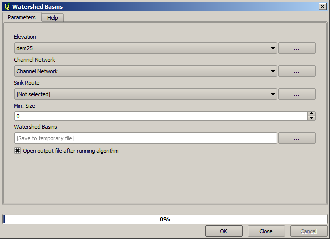
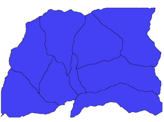
Now, we will use the Watersheds basins algorithm to delineate the subbasins corresponding to that channel network, using as outlet points all the junctions in it. Here is how you have to set the corresponding parameters dialog.
Somit entsteht folgendes.
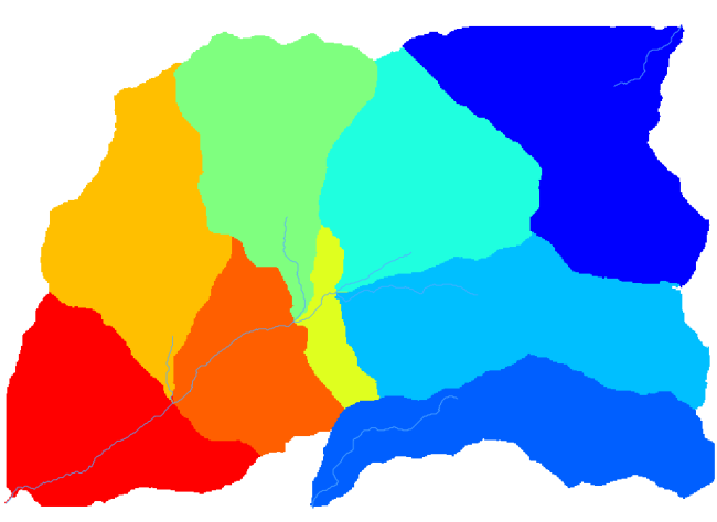
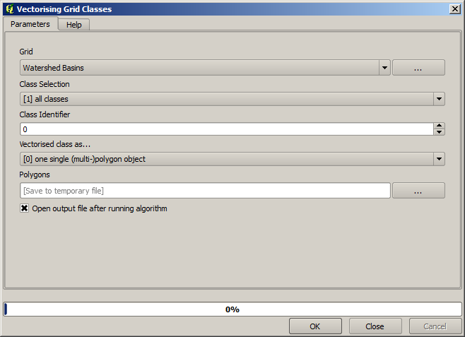
This is a raster result. You can vectorise it using the Vectorising grid classes algorithm.
Nun versuchen wir statistische Höhenwerte in einem unsere Teileinzugsgebiete zu berechnen. Der Gedanke ist einen Layer zu haben, welche stellvertretend für die Höhen im Teileinzugsgebiet steht um dieses an das Modul zu übergeben, welches diese Statistiken berechnet.
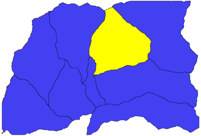
First, let’s clip the original DEM with the polygon representing a subbasin. We will use the Clip raster with polygon algorithm. If we select a single subbasin polygon and then call the clipping algorithm, we can clip the DEM to the area covered by that polygon, since the algorithm is aware of the selection.
Select a polygon
Call the clipping algorithm with the following parameters:
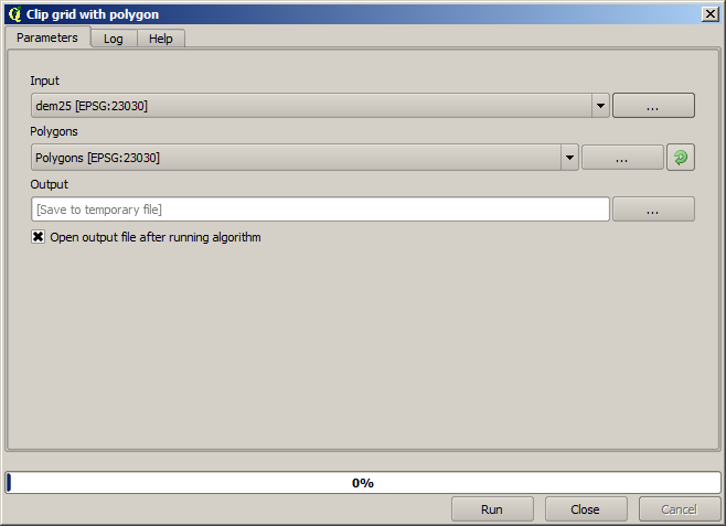
The element selected in the input field is, of course, the DEM we want to clip.
Dies sollte dann in etwa so aussehen.
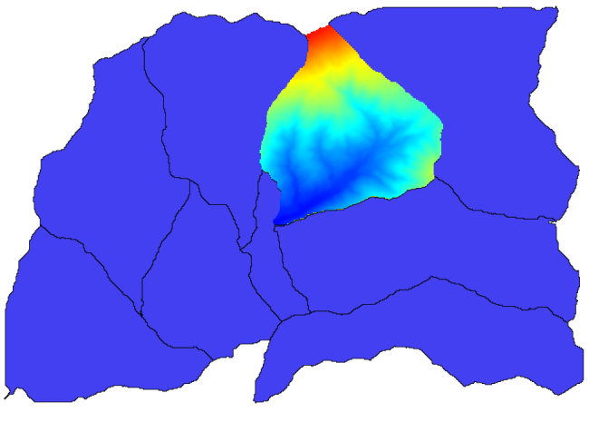
This layer is ready to be used in the Raster layer statistics algorithm.
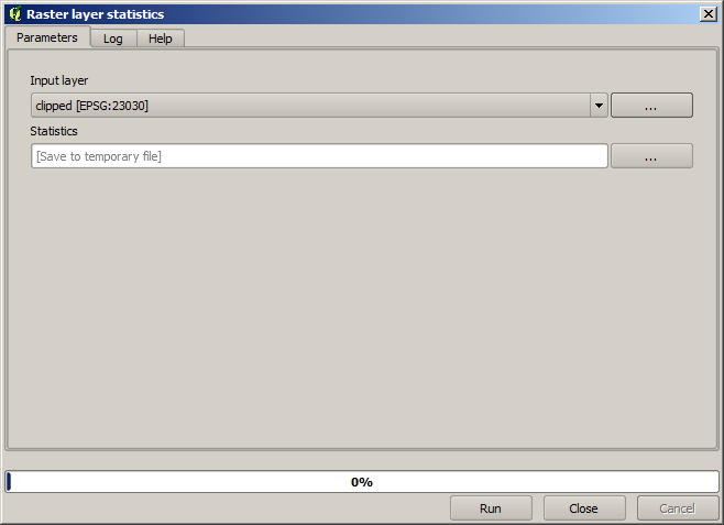
Die resultierende Statistik ist folgende.
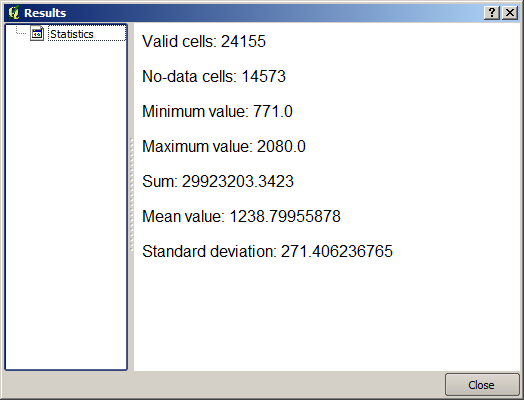
Wir werden die Einzugsgebietsberechnung und die statistischen Werte in einer anderen Übung nochmals verwenden, um herauszufinden wie andere Elemente uns helfen, automatisiert dies durchzuführen und effektiver zu arbeiten.