5.1. Lesson: Creando un Nuevo Conjunto de Datos Vectoriales

Los datos que has usado vienen de algún sitio. Para la mayoría de aplicaciones comunes, los datos ya existen; pero cuanto más particular y especializado sea el proyecto, más difícil será encontrar datos disponibles. En estos casos, necesitarás crear tus propios datos nuevos.

El objetivo de esta lección: Crear un nuevo conjunto de datos.

5.1.1. Follow Along: Cuadro de Diálogo de Creación de Capas

Antes de poder añadir nuevos datos vectoriales, necesitas un conjunto de datos vectoriales al que añadirlos. En nuestro caso, empezarás creando nuevos datos por completo, en lugar de editar un conjunto de datos existente. Además, necesitarás definir de antemano tu propio conjunto de datos nuevo.

Open QGIS and create a new blank project.
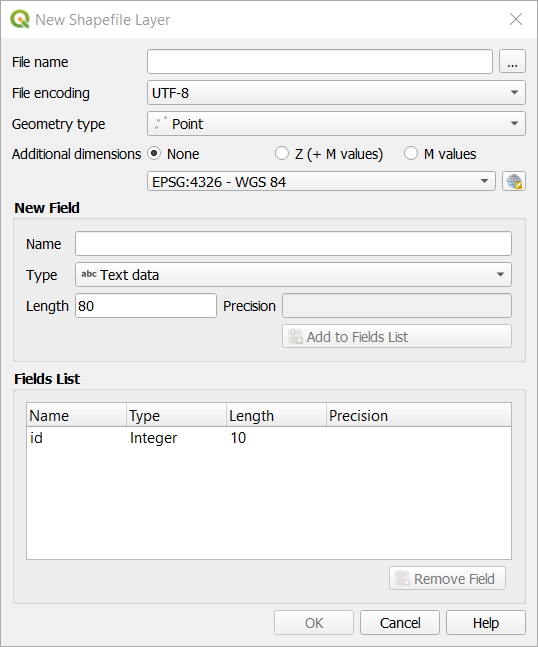
Navigate to and click on the menu entry Layer ► Create Layer ► New Shapefile Layer. You’ll be presented with the New Shapefile Layer dialog, which will allow you to define a new layer.
Click … for the File name field. A save dialog will appear.
Navigate to the exercise_data directory.
Save your new layer as school_property.shp.

Es importante decidir qué tipo de conjunto de datos quieres en este punto. Cada tipo de capa vectorial esta “construida de forma diferente” en sus bases, así que una vez hayas creado la capa, no puedes cambiar su tipo.

For the next exercise, we’re going to create new features which describe areas. For such features, you’ll need to create a polygon dataset.
For Geometry Type, select Polygon from the drop down menu:

Esto no tiene impaco en el resto del cuadro de diálogo, pero hará que se use el tipo correcto de geometría cuando el conjunto de datos vectorial se cree.

The next field allows you to specify the Coordinate Reference System, or CRS. CRS is a method of associating numerical coordinates with a position on the surface of the Earth. See the User Manual on Working with Projections to learn more.

For this example we will use the default CRS associated with this project, which is WGS84.

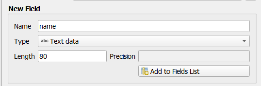
Next there is a collection of fields grouped under New Field. By default, a new layer has only one attribute, the id field (which you should see in the Fields list) below. However, in order for the data you create to be useful, you actually need to say something about the features you’ll be creating in this new layer. For our current purposes, it will be enough to add one field called name that will hold Text data and will be limited to text length of 80 characters.
Replicate the setup below, then click the Add to Fields List button:
Comprueba que tu cuadro de diálogo ahora tiene este aspecto:
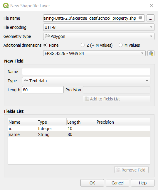
Clique OK.

A nova camada deve aparecer no seu painel Camadas.

5.1.2. Follow Along: Fuentes de Datos

Cuando creas nuevos datos, obviamente deben ser sobre objetos que existen realmente en el terreno. Además, necesitarás obtener la información de alguna parte.

Hay muchas formas posibles de obtener datos sobre objetos. Por ejemplo, podrías utilizar un GPS para capturar puntos en el mundo real y luego importar los datos al QGIS. O podrías sondear los puntos con un teodolito e introducir las coordenadas manualmente para crear nuevas características. También podrías digitalizar procesos para trazar objetos desde sensores de datos remotos, como imagenes de satélite o fotografía aérea.

Para nuestro ejemplo, estarás utilizando un enfoque de digitalización. Las muestras de bases de datos raster se proporcionan, así que necesitarás importarlas cuando sea necesario.

Click on ^{Data Source Manager} button.
Select Raster on the left side.
In the Source panel, click on the … button:
Navigate to exercise_data/raster/.
Select the file 3420C_2010_327_RGB_LATLNG.tif.
Click Open to close the dialogue window.
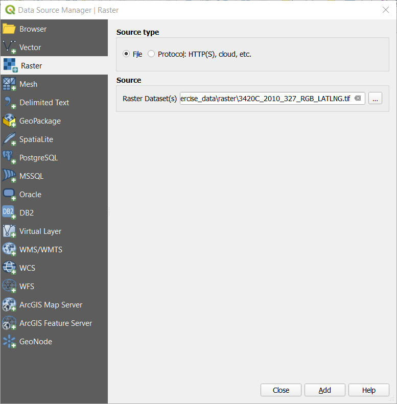
Click Add and Close. An image will load into your map.
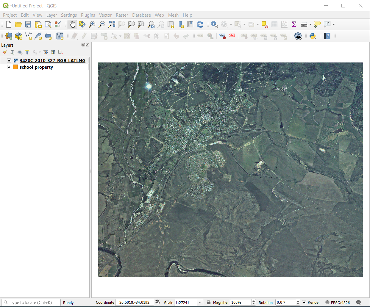
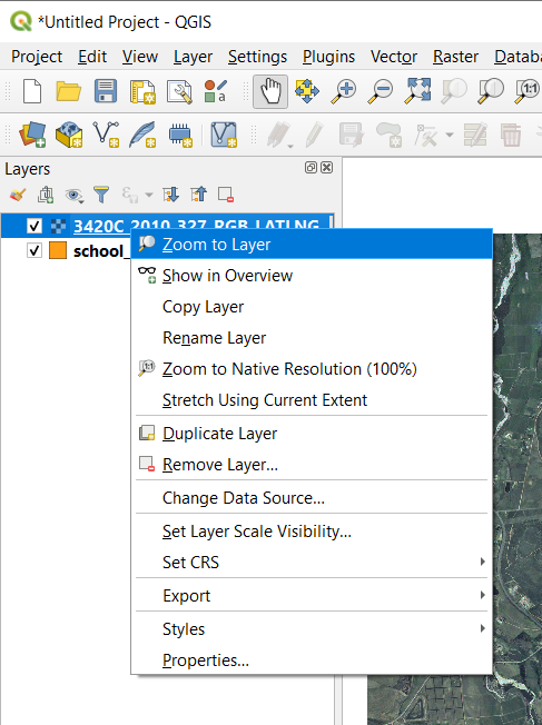
If you don’t see an aerial image appear, select the new layer, right click, and choose Zoom to Layer in the context menu.
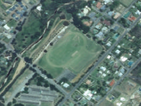
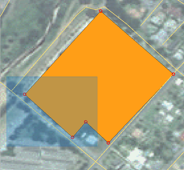
Click on the ^{Zoom In} button, and zoom to the area highlighted in blue below:

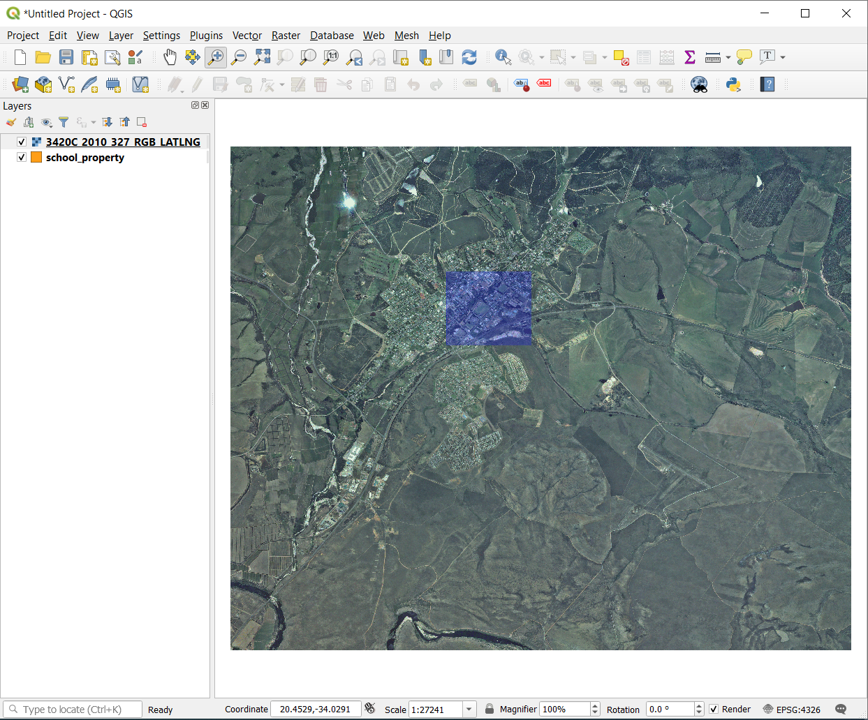
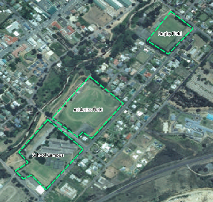
Now you are ready to digitize these three fields:

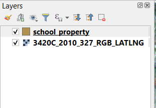
Before starting to digitize, let’s move the school_property layer above the aerial image.

Select school_property layer in the Layers pane and drag it to the top.

Para empezar a digitalizar, necesitarás introducir modo de edición. Los software SIG normalmente lo requieren para prevenir que edites o borres accidentalmente datos importantes. El modo edición se activa o desactiva individualmente para cada capa.

To enter edit mode for the school_property layer:

Click on the school_property layer in the Layers panel to select it.
Click on the ^{Toggle Editing} button.

Si no puedes encontrar ese botón, comprueba que la barra de herramientas Digitalización está activada. Debería haver un marcador junto a la entrada del menú Ver ► Barras de herramientas ► Digitalización.

As soon as you are in edit mode, you’ll see that some digitizing tools have become active:
- ^{Capture Polygon}
- ^{Vertex Tool}
Other relevant buttons are still inactive, but will become active when we start interacting with our new data.

Notice that the layer school_property in the Layers panel now has the pencil icon, indicating that it is in edit mode.
Click on the ^{Capture Polygon} button to begin digitizing our school fields.

You’ll notice that your mouse cursor has become a crosshair. This allows you to more accurately place the points you’ll be digitizing. Remember that even when you’re using the digitizing tool, you can zoom in and out on your map by rolling the mouse wheel, and you can pan around by holding down the mouse wheel and dragging around in the map.

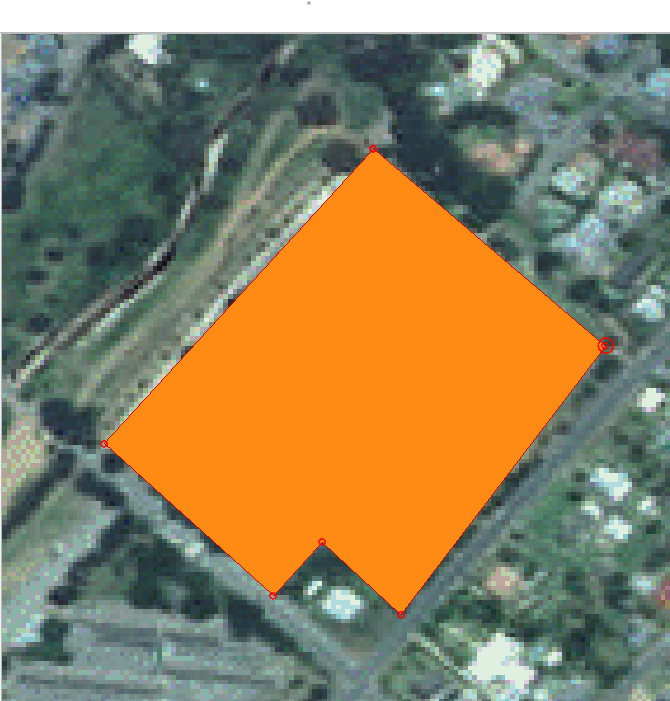
El primer elemento que digitalizarás será el athletics field:
Empieza a digitalizar clicando en un punto a lo largo del borde del campo.
Sitúa más puntos clicando puntos adicionales en el borde, hasta que la forma que estés dibujando cubra completamente el campo.
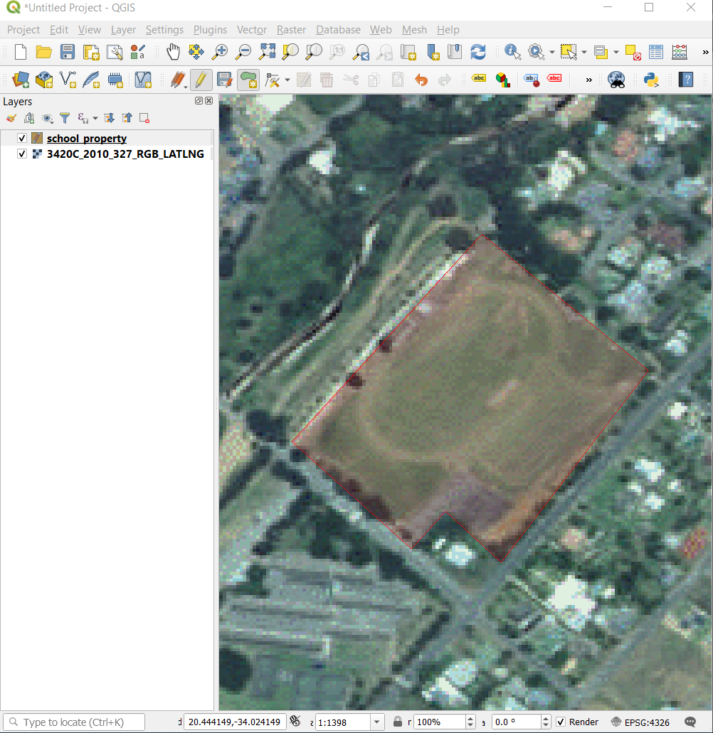
After placing your last point, right click to finish drawing the polygon. This will finalize the feature and show you the Attributes dialog.
Rellena los valores como sigue:
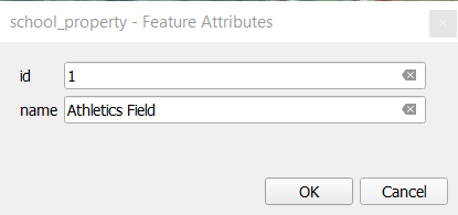
Click OK, and you have created a new feature!
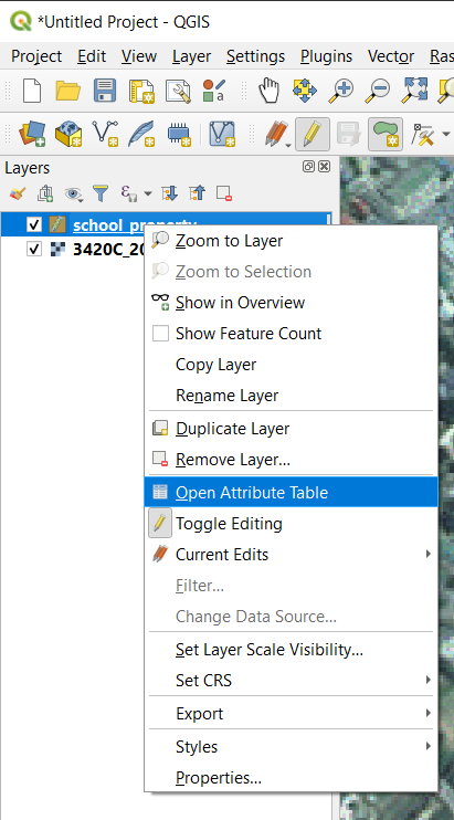
In the Layers panel select the school_property layer.
Right click and choose Open Attribute Table in the context menu.

In the table you will see the feature you just added. While in edit mode you can update the attributes data by double click on the cell you want to update.
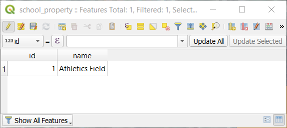
Cierra la tabla de atributos.
To save the new feature we just created, click on ^{Save Edits} button.

Recuerda, si has cometido un error cuando digitalizabas el elemento, siempre puedes editarlo después de haberlo creado. Si has cometido un error, continúa digitalizando hasta que termines de crear el elemento como hasta ahora. Entonces:

Click on ^{Vertex Tool} button.
Hover the mouse over a vertex you want to move and left click on the vertex.
Move the mouse to the correct location of the vertex, and left click. This will move the vertex to the new location.

The same procedure can be used to move a line segment, but you will need to hover over the midpoint of the line segment.

If you want to undo a change, you can press the ^Undo button or Ctrl+Z.
Remember to save your changes by clicking the ^{Save Edits} button.
When done editing, click the ^{Toggle Editing} button to get out of edit mode.

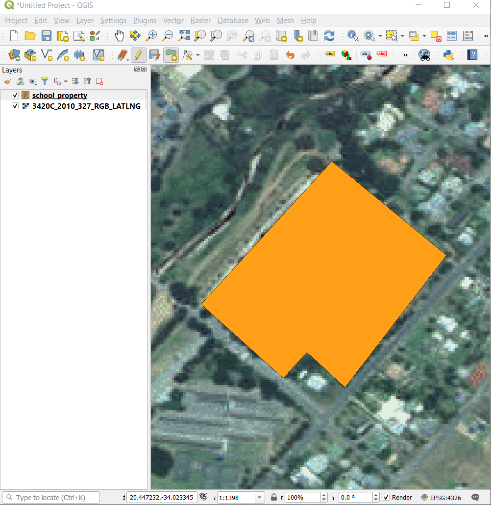
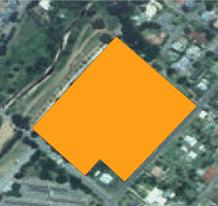
5.1.3. Try Yourself Digitizing Polygons

Digitaliza la propia escuela y el campo superior. Utiliza esta imagen para asistirte:

Remember that each new feature needs to have a unique id value!

Nota

Cuando hayas terminado de añadir elementos a la capa, recuerda guardar tus ediciones y salir del modo edición.

Nota

You can style the fill, outline and label placement and formatting of the school_property using techniques learnt in earlier lessons.

5.1.4. Follow Along: Using Vertex Editor Table

Another way to edit a feature is to manually enter the actual coordinate values for each vertex using the Vertex Editor table.

Make sure you are in edit mode on layer school_property.
If not already activated, click on ^{Vertex Tool} button.
Move the mouse over one of the polygon features you created in the school_property layer and right click on it. This will select the feature and a Vertex Editor pane will appear.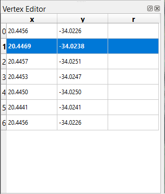

Nota

This table contains the coordinates for the vertices of the feature. Notice there are seven vertices for this feature, but only six are visually identified in the map area. Upon closer inspection, one will notice that row 0 and 6 have identical coordinates. These are the start and end vertices of the feature geometry, and are required in order to create a closed polygon feature.
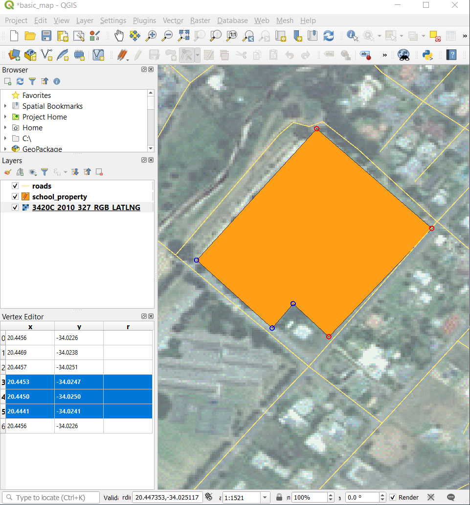
Click and drag a box over a vertex, or multiple vertices, of the selected feature.

The selected vertices will change to a color blue and the Vertex Editor table will have the corresponding rows highlighted, which contain the coordinates of the vertices.
To update a coordinate, double left click on the cell in the table that you want to edit and enter the updated value. In this example, the x coordinate of row 4 is updated from 20.4450 to 20.4444.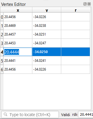
After entering the updated value, hit the enter key to apply the change. You will see the vertex move to the new location in the map window.
When done editing, click the ^{Toggle Editing} button to get out of edit mode, and save your edits.

5.1.5. Try Yourself Digitizing Lines

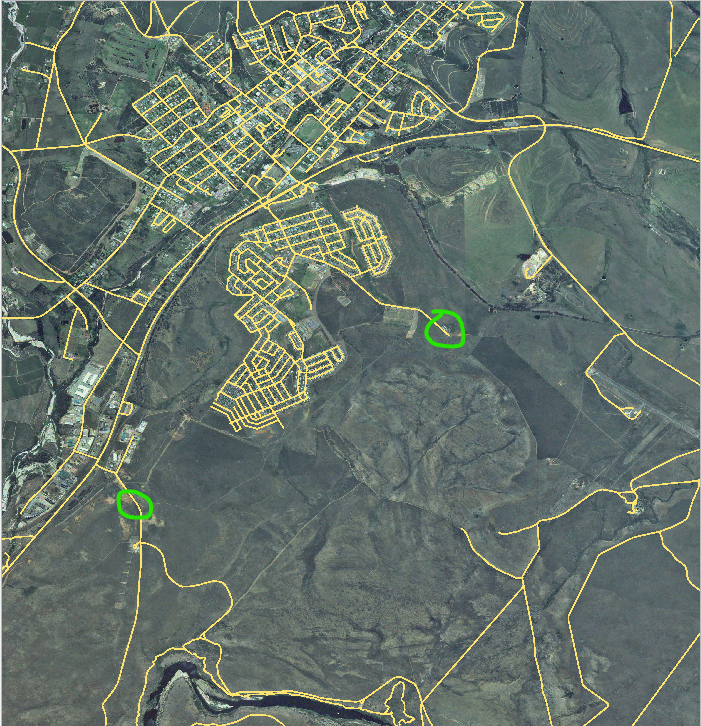
We are going to digitize two routes which are not already marked on the roads layer; one is a path, the other is a track. Our path runs along the southern edge of the suburb of Railton, starting and ending at marked roads:

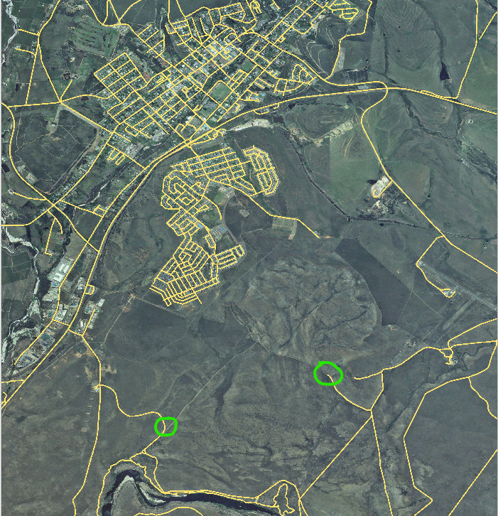
Nuestra pista está un poco más lejos hacia el sur:

If the roads layer is not yet in your map, then add the roads layer from the GeoPackage file training-data.gpkg included in the exercise_data folder of the training data you downloaded. You can read Follow Along: Loading vector data from a GeoPackage Database for a how-to.
Create a new ESRI Shapefile line dataset called routes.shp in the exercise_data directory, with attributes id and type (use the approach above to guide you.)
Activate edit mode on the routes layer.
Since you are working with a line feature, click on the ^{Add Line} button to initiate line digitizing mode.
One at a time, digitize the path and the track on the routes layer. Try to follow the routes as accurately as possible, adding additional points along corners or turns.
Set the type attribute value to path or track.
Use the Layer Properties dialog to add styling to your routes. Feel free to use different styles for paths and tracks.
Save your edits and toggle off editing mode by pressing the ^{Toggle Editing} button.

Comprueba tus resultados

5.1.6. In Conclusion

¡Ahora sabes cómo crear elementos! Este curso no cubre el añadir elementos de tipo puntos, esto no es realmente necesario una vez que has trabajado con elementos más complicados (líneas y polígonos). Funciona exactamente igual, excepto por que solo clicas una vez donde quieras que esté el punto, le das atributos como habitualmente, y luego el elemento se crea.

Saber cómo digitalizar es importante porque es una actividad muy común en programas SIG.

5.1.7. What’s Next?

Features in a GIS layer aren’t just pictures, but objects in space. For example, adjacent polygons know where they are in relation to one another. This is called topology. In the next lesson you’ll see an example of why this can be useful.