15.3. Georeferencer

Wie benutzt man den Georeferenzierer

The Georeferencer is a tool for generating world files for rasters. It allows you to reference rasters to geographic or projected coordinate systems by creating a new GeoTiff or by adding a world file to the existing image. The basic approach to georeferencing a raster is to locate points on the raster for which you can accurately determine coordinates.

Funktionen

Icon	Funktion	Icon	Funktion
	Raster öffnen		Georeferenzierung durchführen
	GDAL-Skript erzeugen		Passpunkte laden
	Passpunkte speichern		Transformationseinstellungen
	Passpunkt hinzufügen		Passpunkt löschen
	Passpunkt verschieben		Verschieben
	Hinein zoomen		Heraus zoomen
	Auf den Layer zoomen		Zoom zurück
	Zoom vor		Georeferenzierung mit QGIS verbinden
	QGIS mit Georeferenzierung verbinden		Volle Histogrammstreckung
	Lokale Histogrammstreckung

Table Georeferenzierung 1: Georeferenzierfunktionen

15.3.1. Wie benutzt man den Georeferenzierer 

As X and Y coordinates (DMS (dd mm ss.ss), DD (dd.dd) or projected coordinates (mmmm.mm)), which correspond with the selected point on the image, two alternative procedures can be used:

The raster itself sometimes provides crosses with coordinates „written“ on the image. In this case, you can enter the coordinates manually.
Using already georeferenced layers. This can be either vector or raster data that contain the same objects/features that you have on the image that you want to georeference and with the projection that you want for your image. In this case, you can enter the coordinates by clicking on the reference dataset loaded in the QGIS map canvas.

The usual procedure for georeferencing an image involves selecting multiple points on the raster, specifying their coordinates, and choosing a relevant transformation type. Based on the input parameters and data, the Georeferencer will compute the world file parameters. The more coordinates you provide, the better the result will be.

The first step is to start QGIS and click on Raster ► Georeferencer, which appears in the QGIS menu bar. The Georeferencer dialog appears as shown in Abb. 15.20.

For this example, we are using a topo sheet of South Dakota from SDGS. It can later be visualized together with the data from the GRASS spearfish60 location. You can download the topo sheet here: https://grass.osgeo.org/sampledata/spearfish_toposheet.tar.gz.

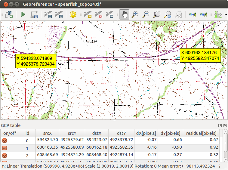
../../../_images/georef.png — Abb. 15.20 Georeferencer Dialog

15.3.1.1. Entering ground control points (GCPs)

To start georeferencing an unreferenced raster, we must load it using the button. The raster will show up in the main working area of the dialog. Once the raster is loaded, we can start to enter reference points.
Using the ^{Add Point} button, add points to the main working area and enter their coordinates (see Figure Abb. 15.21). For this procedure you have three options:
- Click on a point in the raster image and enter the X and Y coordinates manually.
- Click on a point in the raster image and choose the ^{From map canvas} button to add the X and Y coordinates with the help of a georeferenced map already loaded in the QGIS map canvas.
- With the button, you can move the GCPs in both windows, if they are at the wrong place.
Continue entering points. You should have at least four points, and the more coordinates you can provide, the better the result will be. There are additional tools for zooming and panning the working area in order to locate a relevant set of GCP points.

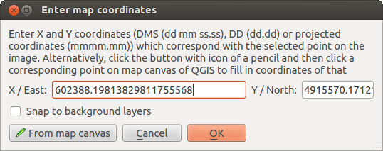
../../../_images/choose_points.png — Abb. 15.21 Add points to the raster image

The points that are added to the map will be stored in a separate text file ([filename].points) usually together with the raster image. This allows us to reopen the Georeferencer at a later date and add new points or delete existing ones to optimize the result. The points file contains values of the form: mapX, mapY, pixelX, pixelY. You can use the ^{Load GCP points} and ^{Save GCP points as} buttons to manage the files.

15.3.1.2. Defining the transformation settings 

After you have added your GCPs to the raster image, you need to define the transformation settings for the georeferencing process.

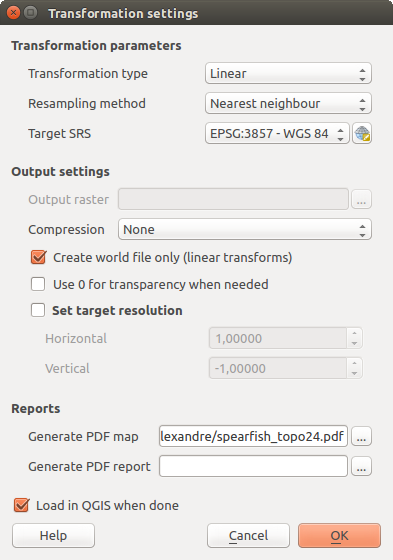
../../../_images/transformation_settings.png — Abb. 15.22 Defining the georeferencer transformation settings

Available Transformation algorithms 

A number of transformation algorithms are available, dependent on the type and quality of input data, the nature and amount of geometric distortion that you are willing to introduce to the final result, and the number of ground control points (GCPs).

Currently, the following Transformation types are available:

The Linear algorithm is used to create a world file and is different from the other algorithms, as it does not actually transform the raster pixels. It allows positioning (translating) the image and uniform scaling, but no rotation or other transformations. It is the most suitable if your image is a good quality raster map, in a known CRS, but is just missing georeferencing information. At least 2 GCPs are needed.
The Helmert transformation also allows rotation. It is particularly useful if your raster is a good quality local map or orthorectified aerial image, but not aligned with the grid bearing in your CRS. At least 2 GCPs are needed.
The Polynomial 1 algorithm allows a more general affine transformation, in particular also a uniform shear. Straight lines remain straight (i.e., collinear points stay collinear) and parallel lines remain parallel. This is particularly useful for georeferencing data cartograms, which may have been plotted (or data collected) with different ground pixel sizes in different directions. At least 3 GCP’s are required.
The Polynomial algorithms 2-3 use more general 2nd or 3rd degree polynomials instead of just affine transformation. This allows them to account for curvature or other systematic warping of the image, for instance photographed maps with curving edges. At least 6 (respectively 10) GCP’s are required. Angles and local scale are not preserved or treated uniformly across the image. In particular, straight lines may become curved, and there may be significant distortion introduced at the edges or far from any GCPs arising from extrapolating the data-fitted polynomials too far.
The Projective algorithm generalizes Polynomial 1 in a different way, allowing transformations representing a central projection between 2 non-parallel planes, the image and the map canvas. Straight lines stay straight, but parallelism is not preserved and scale across the image varies consistently with the change in perspective. This transformation type is most useful for georeferencing angled photographs (rather than flat scans) of good quality maps, or oblique aerial images. A minimum of 4 GCPs is required.
Finally, the Thin Plate Spline (TPS) algorithm „rubber sheets“ the raster using multiple local polynomials to match the GCPs specified, with overall surface curvature minimized. Areas away from GCPs will be moved around in the output to accommodate the GCP matching, but will otherwise be minimally locally deformed. TPS is most useful for georeferencing damaged, deformed, or otherwise slightly inaccurate maps, or poorly orthorectified aerials. It is also useful for approximately georeferencing and implicitly reprojecting maps with unknown projection type or parameters, but where a regular grid or dense set of ad-hoc GCPs can be matched with a reference map layer. It technically requires a minimum of 10 GCPs, but usually more to be successful.

In all of the algorithms except TPS, if more than the minimum GCPs are specified, parameters will be fitted so that the overall residual error is minimized. This is helpful to minimize the impact of registration errors, i.e. slight imprecisions in pointer clicks or typed coordinates, or other small local image deformations. Absent other GCPs to compensate, such errors or deformations could translate into significant distortions, especially near the edges of the georeferenced image. However, if more than the minimum GCPs are specified, they will match only approximately in the output. In contrast, TPS will precisely match all specified GCPs, but may introduce significant deformations between nearby GCPs with registration errors.

Define the Resampling method 

The type of resampling you choose will likely depend on your input data and the ultimate objective of the exercise. If you don’t want to change statistics of the raster (other than as implied by nonuniform geometric scaling if using other than the Linear, Helmert, or Polynomial 1 transformations), you might want to choose ‚Nearest neighbour‘. In contrast, ‚cubic resampling‘, for instance, will usually generate a visually smoother result.

It is possible to choose between five different resampling methods:

Nearest neighbour
Linear
Kubisch
Cubic Spline
Lanczos

Define the transformation settings 

There are several options that need to be defined for the georeferenced output raster.

The Create world file checkbox is only available if you decide to use the linear transformation type, because this means that the raster image actually won’t be transformed. In this case, the Output raster field is not activated, because only a new world file will be created.
For all other transformation types, you have to define an Output raster. As default, a new file ([filename]_modified) will be created in the same folder together with the original raster image.
As a next step, you have to define the Target SRS (Spatial Reference System) for the georeferenced raster (see Arbeiten mit Projektionen).
If you like, you can generate a pdf map and also a pdf report. The report includes information about the used transformation parameters, an image of the residuals and a list with all GCPs and their RMS errors.
Furthermore, you can activate the Set Target Resolution checkbox and define the pixel resolution of the output raster. Default horizontal and vertical resolution is 1.
The Use 0 for transparency when needed can be activated, if pixels with the value 0 shall be visualized transparent. In our example toposheet, all white areas would be transparent.
Finally, Load in QGIS when done loads the output raster automatically into the QGIS map canvas when the transformation is done.

15.3.1.3. Show and adapt raster properties 

Clicking on the Raster properties option in the Settings menu opens the Layer properties dialog of the raster file that you want to georeference.

15.3.1.4. Configure the georeferencer 

You can define whether you want to show GCP coordinates and/or IDs.
As residual units, pixels and map units can be chosen.
For the PDF report, a left and right margin can be defined and you can also set the paper size for the PDF map.
Finally, you can activate to Show Georeferencer window docked.

15.3.1.5. Running the transformation 

After all GCPs have been collected and all transformation settings are defined, just press the ^{Start georeferencing} button to create the new georeferenced raster.