22.5. The graphical modeler
The graphical modeler allows you to create complex models using a simple and easy-to-use interface. When working with a GIS, most analysis operations are not isolated, rather part of a chain of operations. Using the graphical modeler, that chain of operations can be wrapped into a single process, making it convenient to execute later with a different set of inputs. No matter how many steps and different algorithms it involves, a model is executed as a single algorithm, saving time and effort.
The graphical modeler can be opened from the Processing menu ().
The modeler has a working canvas where the structure of the model and the workflow it represents are shown. The left part of the window is a panel with two tabs that can be used to add new elements to the model.
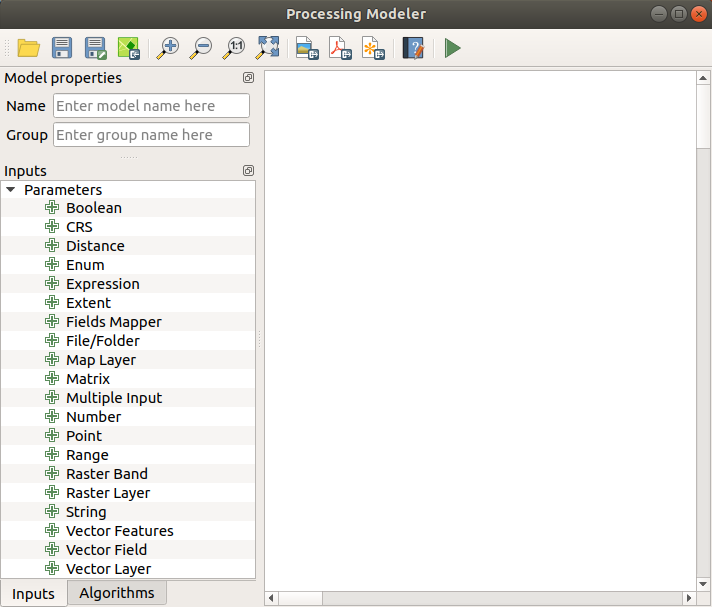
Fig. 22.18 Modeler
Creating a model involves two steps:
Definition of necessary inputs. These inputs will be added to the parameters window, so the user can set their values when executing the model. The model itself is an algorithm, so the parameters window is generated automatically as it happens with all the algorithms available in the processing framework.
Definition of the workflow. Using the input data of the model, the workflow is defined by adding algorithms and selecting how they use the defined inputs or the outputs generated by other algorithms in the model.
22.5.1. Definition of inputs
The first step is to define the inputs for the model. The following elements are found in the Inputs tab on the left side of the modeler window:
Authentication Configuration
Boolean
CRS
Color
Distance
Enum
Expression
Extent
Fields Mapper
File/Folder
Map Layer
Matrix
Multiple Input
Number
Point
Print Layout
Print Layout Item
Range
Raster Band
Raster Layer
Scale
String
Vector Features
Vector Field
Vector Layer
When double-clicking on an element, a dialog is shown that lets you define its characteristics. Depending on the parameter, the dialog will contain at least one basic element (the description, which is what the user will see when executing the model). When adding a numerical value, as can be seen in the next figure, in addition to the description of the parameter, you have to set a default value and the range of valid values.
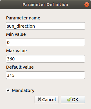
Fig. 22.19 Model Parameters Definition
You can define your input as mandatory for your model by checking the
 Mandatory option and by checking the
  Advanced
checkbox you can set the input to be within the Advanced section.
This is particularly useful when the model has many parameters and some
of them are not trivial, but you still want to choose them.
For each added input, a new element is added to the modeler canvas.
Advanced
checkbox you can set the input to be within the Advanced section.
This is particularly useful when the model has many parameters and some
of them are not trivial, but you still want to choose them.
For each added input, a new element is added to the modeler canvas.

Fig. 22.20 Model Parameters
You can also add inputs by dragging the input type from the list and dropping it in the position where you want it in the modeler canvas.
22.5.2. Definition of the workflow
Once the inputs have been defined, it is time to define the algorithms of the model. Algorithms can be found in the Algorithms tab, grouped much in the same way as they are in the Processing toolbox.
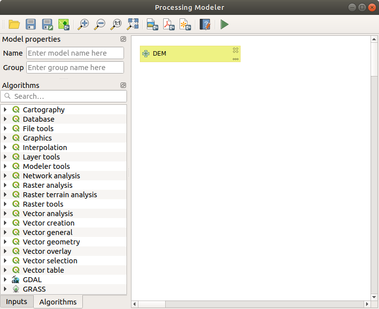
Fig. 22.21 Model Inputs
To add an algorithm to a model, double-click on its name or drag and drop it, just like for inputs. An execution dialog will appear, with a content similar to the one found in the execution panel that is shown when executing the algorithm from the toolbox. The ones shown next correspond to the QGIS ‘Drape (set Z value from raster)’ algorithm and the QGIS ‘Climb along line’ algorithm.
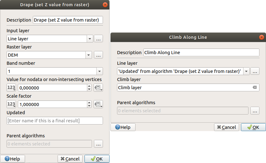
Fig. 22.22 Model Algorithm parameters
As you can see, some differences exist. Instead of the file output box that was used to set the file path for output layers and tables, a simple text box is used here. If the layer generated by the algorithm is just a temporary result that will be used as the input of another algorithm and should not be kept as a final result, just do not edit that text box. Typing anything in it means that the result is final and the text that you supply will be the description for the output, which will be the output the user will see when executing the model.
Selecting the value of each parameter is also a bit different, since there are important differences between the context of the modeler and that of the toolbox. Let’s see how to introduce the values for each type of parameter.
Layers (raster and vector) and tables. These are selected from a list, but in this case, the possible values are not the layers or tables currently loaded in QGIS, but the list of model inputs of the corresponding type, or other layers or tables generated by algorithms already added to the model.
Numerical values. Literal values can be introduced directly in the text box. Clicking on the button beside the text box, expressions can be entered. Available variables for expressions include numerical inputs of the model, outputs from model algorithms and also statistical values from available layers within the model.
String. Literal strings can be typed in the corresponding text box. Clicking on the button beside the text box, expressions can be entered, as for numerical values.
Vector Field. The fields of a vector layer cannot be known at design time, since they depend on the selection of the user each time the model is executed. To set the value for this parameter, type the name of a field directly in the text box, or use the list to select a table field. The validity of the selected field will be checked at run time.
In all cases, you will find an additional parameter named Parent algorithms that is not available when calling the algorithm from the toolbox. This parameter allows you to define the order in which algorithms are executed by explicitly defining one algorithm as a parent of the current one, which will force the parent algorithm to be executed before the current one.
When you use the output of a previous algorithm as the input of your algorithm, that implicitly sets the previous algorithm as parent of the current one (and places the corresponding arrow in the modeler canvas). However, in some cases an algorithm might depend on another one even if it does not use any output object from it (for instance, an algorithm that executes a SQL sentence on a PostGIS database and another one that imports a layer into that same database). In that case, just select the previous algorithm in the Parent algorithms parameter and they will be executed in the correct order.
Once all the parameters have been assigned valid values, click on OK and the algorithm will be added to the canvas. It will be linked to the elements in the canvas (algorithms or inputs) that provide objects that are used as inputs for the algorithm.
Elements can be dragged to a different position on the canvas. This is useful to make the structure of the model more clear and intuitive. Links between elements are updated automatically. You can zoom in and out by using the mouse wheel.
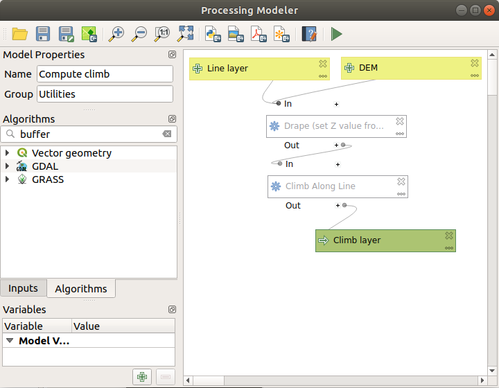
Fig. 22.23 A complete model
You can run your algorithm any time by clicking on the Run button. In order to use the algorithm from the toolbox, it has to be saved and the modeler dialog closed, to allow the toolbox to refresh its contents.
22.5.3. Saving and loading models
Use the Save button to save the current model and the
Open button to open any previously saved model.
Models are saved with the .model3 extension.
If the model has been already been saved from the modeler window,
you will not be prompted for a filename.
Since there is already a file associated with the model, that file
will be used for subsequent saves.
Before saving a model, you have to enter a name and a group for it in the text boxes in the upper part of the window.
Models saved in the models folder (the default folder when you
are prompted for a filename to save the model) will appear in the
toolbox in the corresponding branch.
When the toolbox is invoked, it searches the models folder for
files with the .model3 extension and loads the models they
contain.
Since a model is itself an algorithm, it can be added to the toolbox
just like any other algorithm.
Models can also be saved within the project file using the
 Save model in project button.
Models saved using this method won’t be written as
Save model in project button.
Models saved using this method won’t be written as .model3 files
on the disk but will be embedded in the project file.
Project models are available in the
 Project models menu of the toolbox.
The models folder can be set from the Processing configuration dialog, under the Modeler group.
Models loaded from the models folder appear not only in the
toolbox, but also in the algorithms tree in the Algorithms
tab of the modeler window.
That means that you can incorporate a model as a part of a bigger model,
just like other algorithms.
Models will show up in the Browser panel , and can be run from there.
22.5.3.1. Exporting a model as an image, PDF or SVG
A model can also be exported as an image, SVG or PDF (for illustration purposes).
22.5.4. Editing a model
You can edit the model you are currently creating, redefining the workflow and the relationships between the algorithms and inputs that define the model.
If you right-click on an algorithm in the canvas, you will see a context menu like the one shown next:
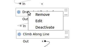
Fig. 22.24 Modeler Right Click
Selecting the Remove option will cause the selected algorithm to be removed. An algorithm can be removed only if there are no other algorithms depending on it. That is, if no output from the algorithm is used in a different one as input. If you try to remove an algorithm that has others depending on it, a warning message like the one you can see below will be shown:
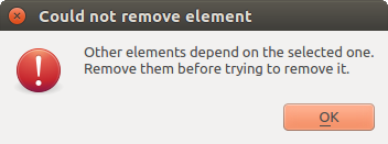
Fig. 22.25 Cannot Delete Algorithm
Selecting the Edit option will show the parameter dialog of the algorithm, so you can change the inputs and parameter values. Not all input elements available in the model will appear as available inputs. Layers or values generated at a more advanced step in the workflow defined by the model will not be available if they cause circular dependencies.
Select the new values and click on the OK button as usual. The connections between the model elements will change in the modeler canvas accordingly.
A model can be run partially, by deactivating some of its algorithms. To do it, select the Deactivate option in the context menu that appears when right-clicking on an algorithm element. The selected algorithm, and all the ones in the model that depend on it will be displayed in grey and will not be executed as part of the model.
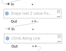
Fig. 22.26 Model With Deactivated Algorithms
When right-clicking on an algorithm that is not active, you will see a Activate menu option that you can use to reactivate it.
22.5.5. Editing model help files and meta-information
You can document your models from the modeler itself. Just click on the Edit Model Help button, and a dialog like the one shown next will appear.
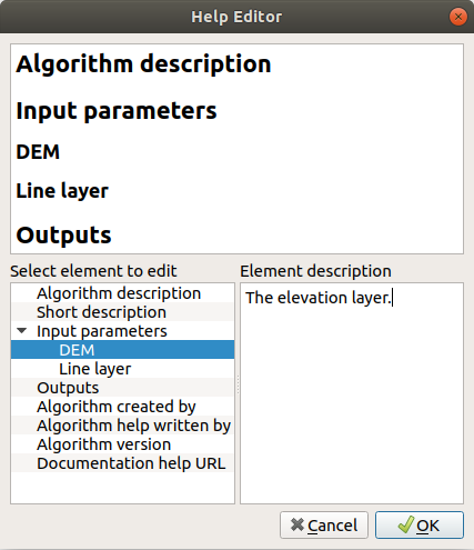
Fig. 22.27 Editing Help
On the right-hand side, you will see a simple HTML page, created using the description of the input parameters and outputs of the algorithm, along with some additional items like a general description of the model or its author. The first time you open the help editor, all these descriptions are empty, but you can edit them using the elements on the left-hand side of the dialog. Select an element on the upper part and then write its description in the text box below.
Model help is saved as part of the model itself.
22.5.6. Exporting a model as a Python script
As we will see in a later chapter, Processing algorithms can be called from the QGIS Python console, and new Processing algorithms can be created using Python. A quick way of creating such a Python script is to create a model and then to export is as a Python file.
To do so, right click on the name of the model in the Processing Toolbox and choose Export Model as Python Algorithm….
22.5.7. About available algorithms
You might notice that some algorithms that can be executed from the toolbox do not appear in the list of available algorithms when you are designing a model. To be included in a model, an algorithm must have the correct semantic. If an algorithm does not have such a well-defined semantic (for instance, if the number of output layers cannot be known in advance), then it is not possible to use it within a model, and it will not appear in the list of algorithms that you can find in the modeler dialog.