22.3. The Toolbox
The Processing Toolbox is the main element of the processing GUI, and the one that you are more likely to use in your daily work. It shows the list of all available algorithms grouped in different blocks called Providers, and custom models and scripts you can add to extend the set of tools. Hence the toolbox is the access point to run them, whether as a single process or as a batch process involving several executions of the same algorithm on different sets of inputs.
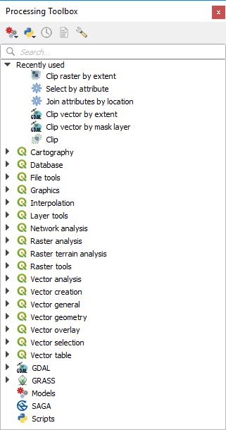
Fig. 22.6 Processing Toolbox
Providers can be (de)activated in the Processing settings dialog. By default, only providers that do not rely on third-party applications (that is, those that only require QGIS elements to be run) are active. Algorithms requiring external applications might need additional configuration. Configuring providers is explained in a later chapter in this manual.
In the upper part of the toolbox dialog, you will find a set of tools to:
work with
 Models: Create New Model…,
Open Existing Model… and Add Model to Toolbox…;
Models: Create New Model…,
Open Existing Model… and Add Model to Toolbox…;work with
 Scripts: Create New Script…,
Create New Script from Template…, Open Existing
Script… and Add Script to Toolbox…;
Scripts: Create New Script…,
Create New Script from Template…, Open Existing
Script… and Add Script to Toolbox…;open the
 History panel;
open the
 Results Viewer panel;
toggle the toolbox to the in-place modification mode using the
 Edit Features In-Place button: only
the algorithms that are suitable to be executed on the active layer without
outputting a new layer are displayed;
Edit Features In-Place button: only
the algorithms that are suitable to be executed on the active layer without
outputting a new layer are displayed;open the
 Options dialog.
Below this toolbar is a  Search… box to help you easily find
the tools you need.
You can enter any word or phrase on the text box. Notice that, as you type, the
number of algorithms, models or scripts in the toolbox is reduced to just those
that contain the text you have entered in their names or keywords.
Search… box to help you easily find
the tools you need.
You can enter any word or phrase on the text box. Notice that, as you type, the
number of algorithms, models or scripts in the toolbox is reduced to just those
that contain the text you have entered in their names or keywords.
Note
At the top of the list of algorithms are displayed the most recent used tools; handy if you want to reexecute any.
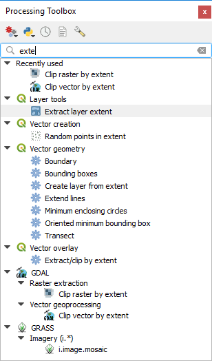
Fig. 22.7 Processing Toolbox showing search results
To execute a tool, just double-click on its name in the toolbox.
22.3.1. The algorithm dialog
Once you double-click on the name of the algorithm that you want to execute, a
dialog similar to that in the figure below is shown (in this case, the dialog
corresponds to the Centroids algorithm).
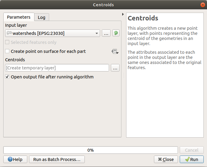
Fig. 22.8 Algorithm Dialog - Parameters
This dialog is used to set the input values that the algorithm needs to be executed. It shows a list of input values and configuration parameters to be set. It of course has a different content, depending on the requirements of the algorithm to be executed, and is created automatically based on those requirements.
Although the number and type of parameters depend on the characteristics of the algorithm, the structure is similar for all of them. The parameters found in the table can be of one of the following types.
A raster layer, to select from a list of all such layers available (currently opened) in QGIS. The selector contains as well a button on its right-hand side, to let you select filenames that represent layers currently not loaded in QGIS.
A vector layer, to select from a list of all vector layers available in QGIS. Layers not loaded in QGIS can be selected as well, as in the case of raster layers, but only if the algorithm does not require a table field selected from the attributes table of the layer. In that case, only opened layers can be selected, since they need to be open so as to retrieve the list of field names available.
You will see an iterator button by each vector layer selector, as shown in the figure below.
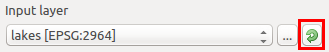
Fig. 22.9 Vector iterator button
If the algorithm contains several of them, you will be able to toggle just one of them. If the button corresponding to a vector input is toggled, the algorithm will be executed iteratively on each one of its features, instead of just once for the whole layer, producing as many outputs as times the algorithm is executed. This allows for automating the process when all features in a layer have to be processed separately.
Note
By default, the parameters dialog will show a description of the CRS of each layer along with its name. If you do not want to see this additional information, you can disable this functionality in the Processing Settings dialog, unchecking the option.
A table, to select from a list of all available in QGIS. Non-spatial tables are loaded into QGIS like vector layers, and in fact they are treated as such by the program. Currently, the list of available tables that you will see when executing an algorithm that needs one of them is restricted to tables coming from files in dBase (
.dbf) or Comma-Separated Values (.csv) formats.An option, to choose from a selection list of possible options.
A numerical value, to be introduced in a spin box. In some contexts (when the parameter applies at the feature level and not at the layer’s), you will find a
 Data-defined override button by its side, allowing
you to open the expression builder and enter a
mathematical expression to generate variable values for the parameter. Some useful
variables related to data loaded into QGIS can be added to your expression, so
you can select a value derived from any of these variables, such as the cell size
of a layer or the northernmost coordinate of another one.
Data-defined override button by its side, allowing
you to open the expression builder and enter a
mathematical expression to generate variable values for the parameter. Some useful
variables related to data loaded into QGIS can be added to your expression, so
you can select a value derived from any of these variables, such as the cell size
of a layer or the northernmost coordinate of another one.
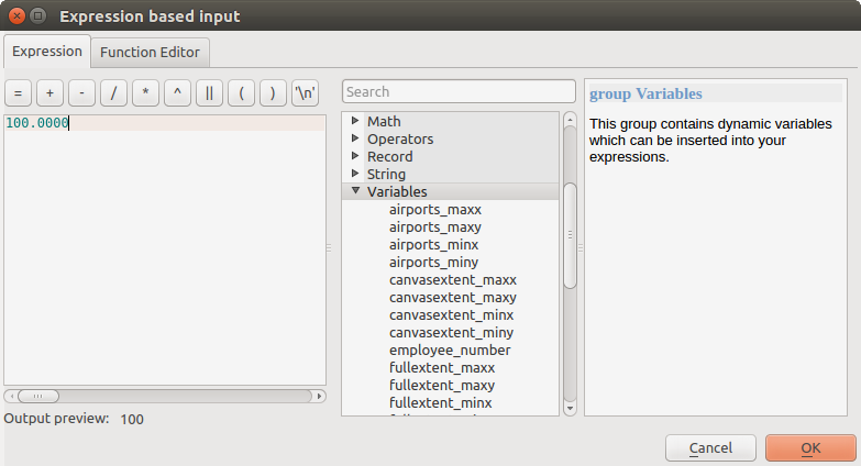
Fig. 22.10 Expression based input
A range, with min and max values to be introduced in two text boxes.
A text string, to be introduced in a text box.
A field, to choose from the attributes table of a vector layer or a single table selected in another parameter.
A coordinate reference system. You can select it among the recently used ones from the drop-down list or from the CRS selection dialog that appears when you click on the button on the right-hand side.
An extent, to be entered by four numbers representing its
xmin,xmax,ymin,ymaxlimits. Clicking on the button on the right-hand side of the value selector, a pop-up menu will appear, giving you options:to select the value from a layer or the current canvas extent;
or to define it by dragging directly onto the map canvas.
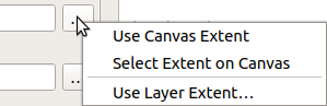
Fig. 22.11 Extent selector
If you select the first option, you will see a window like the next one.
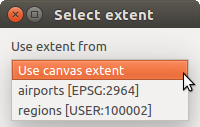
Fig. 22.12 Extent List
If you select the second one, the parameters window will hide itself, so you can click and drag onto the canvas. Once you have defined the selected rectangle, the dialog will reappear, containing the values in the extent text box.
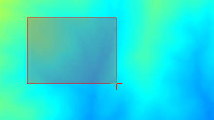
Fig. 22.13 Extent Drag
A list of elements (whether raster or vector layers, tables, fields) to select from. Click on the … button at the left of the option to see a dialog like the following one. Multiple selection is allowed and when the dialog is closed, number of selected items is displayed in the parameter text box widget.
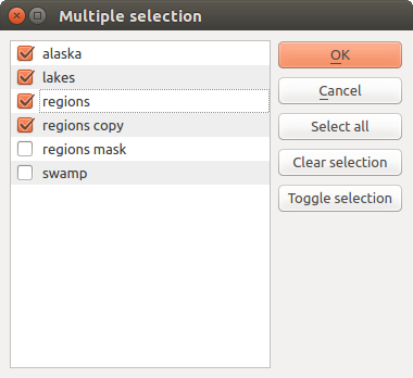
Fig. 22.14 Multiple Selection
A small table to be edited by the user. These are used to define parameters like lookup tables or convolution kernels, among others.
Click on the button on the right side to see the table and edit its values.
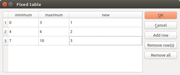
Fig. 22.15 Fixed Table
Depending on the algorithm, the number of rows can be modified or not by using the buttons on the right side of the window.
Note
Some algorithms require many parameter to run, e.g. in the
Raster calculator you have to specify manually the cell size, the
extent and the CRS. You can avoid to choose all the parameters manually when
the algorithm has the Reference layers parameter. With this parameter you
can choose the reference layer and all its properties (cell size, extent, CRS)
will be used.
Along with the Parameters tab, there is another tab named Log (see figure below). Information provided by the algorithm during its execution is written in this tab, and allow you to track the execution and be aware and have more details about the algorithm as it runs. Notice that not all algorithms write information to this tab, and many of them might run silently without producing any output other than the final files.
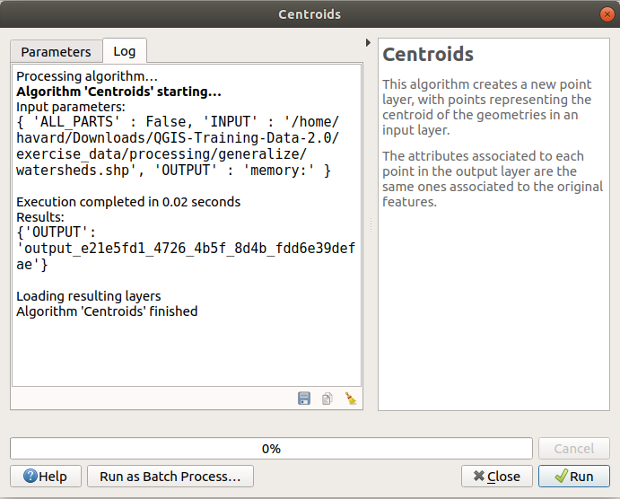
Fig. 22.16 Algorithm Dialog - Log
At the bottom of the Log tab you will find buttons to
Save Log to File, Copy Log to Clipboard and Clear Log.
These are particularly handy when you have checked the
Keep dialog open after running algorithm in the General part
of the Processing options.
On the right hand side of the dialog you will find a short description of the algorithm, which will help you understand its purpose and its basic ideas. If such a description is not available, the description panel will not be shown.
For a more detailed help file, which might include description of every parameter it uses, or examples, you will find a Help button at the bottom of the dialog bringing you to the Processing algorithms documentation or to the provider documentation (for some third-party providers).
22.3.1.1. A note on projections
Processing algorithm execution are always performed in the input layer coordinate reference system (CRS). Due to QGIS’s on-the-fly reprojecting capabilities, although two layers might seem to overlap and match, that might not be true if their original coordinates are used without reprojecting them onto a common coordinate system. Whenever you use more than one layer as input to a QGIS native algorithm, whether vector or raster, the layers will all be reprojected to match the coordinate reference system of the first input layer.
This is however less true for most of the external applications whose algorithms are exposed through the processing framework as they assume that all of the layers are already in a common coordinate system and ready to be analyzed.
By default, the parameters dialog will show a description of the CRS of each layer along with its name, making it easy to select layers that share the same CRS to be used as input layers. If you do not want to see this additional information, you can disable this functionality in the Processing settings dialog, unchecking the Show layer CRS definition in selection boxes option.
If you try to execute an algorithm using as input two or more layers with unmatching CRSs, a warning dialog will be shown. This occurs thanks to the Warn before executing if layer CRS’s do not match option.
You still can execute the algorithm, but be aware that in most cases that will produce wrong results, such as empty layers due to input layers not overlapping.
Tip
Use Processing algorithms to do intermediate reprojection
When an algorithm can not successfully perform on multiple input layers due to unmatching CRSs, use QGIS internal algorithm such as Reproject layer to perform layers’ reprojection to the same CRS before executing the algorithm using these outputs.
22.3.2. Data objects generated by algorithms
Data objects generated by an algorithm can be of any of the following types:
A raster layer
A vector layer
A table
An HTML file (used for text and graphical outputs)
These are all saved to disk, and the parameters table will contain a text box corresponding to each one of these outputs, where you can type the output channel to use for saving it. An output channel contains the information needed to save the resulting object somewhere. In the most usual case, you will save it to a file, but in the case of vector layers, and when they are generated by native algorithms (algorithms not using external applications) you can also save to a PostGIS, GeoPackage or SpatiaLite database, or a memory layer.
To select an output channel, just click on the button on the right side of the text box, and you will see a small context menu with the available options.
In the most usual case, you will select saving to a file. If you select that option, you will be prompted with a save file dialog, where you can select the desired file path. Supported file extensions are shown in the file format selector of the dialog, depending on the kind of output and the algorithm.
The format of the output is defined by the filename extension. The supported
formats depend on what is supported by the algorithm itself. To select a format,
just select the corresponding file extension (or add it, if you are directly typing
the file path instead). If the extension of the file path you entered does not
match any of the supported formats, a default extension will be
appended to the file path, and the file format corresponding to that extension will
be used to save the layer or table. Default extensions are .dbf for
tables, .tif for raster layers and .gpkg for vector layers. These
can be modified in the setting dialog, selecting any other of the formats supported
by QGIS.
If you do not enter any filename in the output text box (or select the corresponding option in the context menu), the result will be saved as a temporary file in the corresponding default file format, and it will be deleted once you exit QGIS (take care with that, in case you save your project and it contains temporary layers).
You can set a default folder for output data objects. Go to the settings
dialog (you can open it from the
menu), and in the
General group, you will find a parameter named Output folder.
This output folder is used as the default path in case you type just a filename
with no path (i.e., myfile.shp) when executing an algorithm.
When running an algorithm that uses a vector layer in iterative mode, the entered file path is used as the base path for all generated files, which are named using the base name and appending a number representing the index of the iteration. The file extension (and format) is used for all such generated files.
Apart from raster layers and tables, algorithms also generate graphics and text as HTML files. These results are shown at the end of the algorithm execution in a new dialog. This dialog will keep the results produced by any algorithm during the current session, and can be shown at any time by selecting from the QGIS main menu.
Some external applications might have files (with no particular extension restrictions) as output, but they do not belong to any of the categories above. Those output files will not be processed by QGIS (opened or included into the current QGIS project), since most of the time they correspond to file formats or elements not supported by QGIS. This is, for instance, the case with LAS files used for LiDAR data. The files get created, but you won’t see anything new in your QGIS working session.
For all the other types of output, you will find a checkbox that you can use to tell the algorithm whether to load the file once it is generated by the algorithm or not. By default, all files are opened.
Optional outputs are not supported. That is, all outputs are created. However, you can uncheck the corresponding checkbox if you are not interested in a given output, which essentially makes it behave like an optional output (in other words, the layer is created anyway, but if you leave the text box empty, it will be saved to a temporary file and deleted once you exit QGIS).