17.5. Mai multe tipuri de date și algoritmi
Notă
În această lecție vom rula mai mult de trei algoritmi, veți învăța cum să folosiți alte tipuri de intrări, și cum să configurați rezultatele pentru a fi salvate automat într-un anumit folder.
Pentru aceste lecții vom avea nevoie de o tabelă și de un strat poligonal. Vom crea un strat de puncte bazat pe coordonatele din tabel, și apoi vom contoriza numărul de puncte din fiecare poligon. Dacă deschideți proiectul QGIS corespunzător acestei lecții, veți găsi un tabel cu coordonatele X și Y, dar veți identifica nici un strat poligonal. Nu vă faceți griji, îl vom crea folosind un geoalgoritm de procesare.
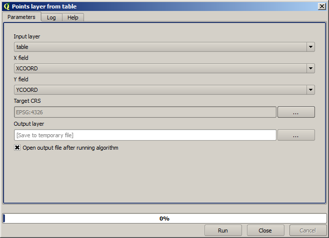
Primul lucru pe care îl vom face este de a crea un strat de puncte din coordonatele din tabel, utilizând algoritmul Stratului de puncte din tabelă. O dată ce știți cum se folosește caseta de căutare, nu vă va fi greu să-l găsiți. Efectuați un dublu-clic pe ea pentru a o rula și pentru a ajunge la următorul său dialog.
Acest algoritm, la fel ca și cel din lecția precedentă, generează doar o singură ieșire, având trei intrări:
Tabela: tabela cu coordonate. Ar trebui să selectați aici tabela corespunzătoare lecției.
X and Y fields: these two parameters are linked to the first one. The corresponding selector will show the name of those fields that are available in the selected table. Select the XCOORD field for the X parameter, and the YYCOORD field for the Y parameter.
CRS: Since this algorithm takes no input layers, it cannot assign a CRS to the output layer based on them. Instead, it asks you to manually select the CRS that the coordinates in the table use. Click on the button on the left–hand side to open the QGIS CRS selector, and select EPSG:4326 as the output CRS. We are using this CRS because the coordinates in the table are in that CRS.
Dialogul dvs. ar trebui să arate astfel.
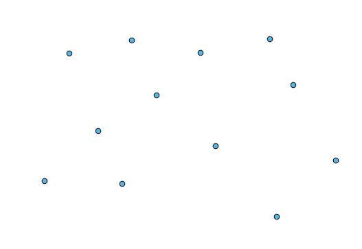
Now press the Run button to get the following layer (you may need to zoom full to reenter the map around the newly created points):
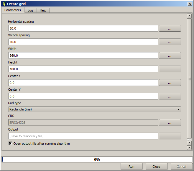
Următorul lucru de care avem nevoie este stratul poligona;. Vom crea o grilă obișnuită de poligoane, folosind algoritmul Creare grilă, care are următoarea fereastră cu parametri.
Atenționare
The options are simpler in recent versions of QGIS; you just need to enter min and max for X and Y (suggested values: -5.696226,-5.695122,40.24742,40.248171)
The inputs required to create the grid are all numbers. When you have to enter a numerical value, you have two options: typing it directly on the corresponding box or clicking the button on the right–hand side to get to a dialog like the one shown next.
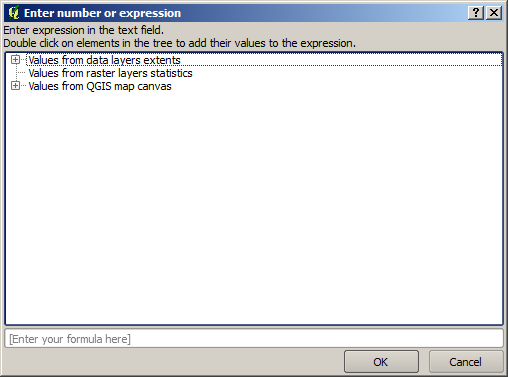
The dialog contains a simple calculator, so you can type expressions such as 11 * 34.7 + 4.6, and the result will be computed and put in the corresponding text box in the parameters dialog. Also, it contains constants that you can use, and values from other layers available.
In this case, we want to create a grid that covers the extent of the input points layer, so we should use its coordinates to calculate the center coordinate of the grid and its width and height, since those are the parameters that the algorithm takes to create the grid. With a little bit of math, try to do that yourself using the calculator dialog and the constants from the input points layer.
Selectați Dreptunghiuri (poligoane) în câmpul Tip.
As in the case of the last algorithm, we have to enter the CRS here as well. Select EPSG:4326 as the target CRS, as we did before.
În cele din urmă, ar trebui să aveți un dialog pentru parametri de genul următor:
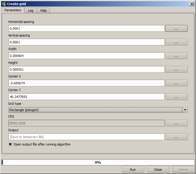
(Better add one spacing on the width and height: Horizontal spacing: 0.0001, Vertical spacing: 0.0001, Width: 0.001004, Height: 0.000651, Center X: -5.695674, Center Y: 40.2477955) The case of X center is a bit tricky, see: -5.696126+(( -5.695222+ 5.696126)/2)
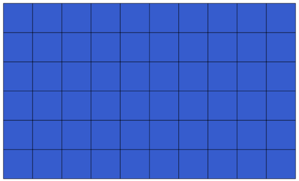
Apăsați Run pentru a obține stratul de graticule.
The last step is to count the points in each one of the rectangles of that graticule. We will use the Count points in polygons algorithm.
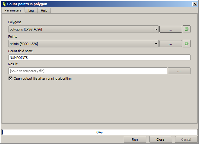
Acum avem rezultatul dorit.
Before finishing this lesson, here is a quick tip to make your life easier in case you want to persistently save your data. If you want all your output files to be saved in a given folder, you do not have to type the folder name each time. Instead, go to the processing menu and select the Options and configuration item. It will open the configuration dialog.
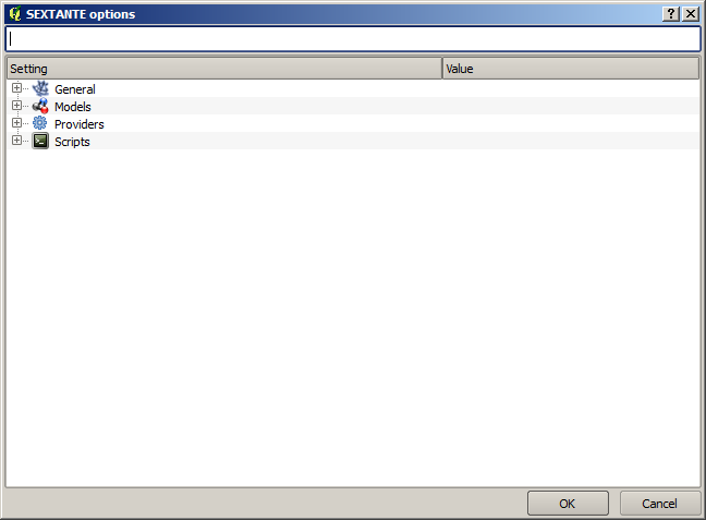
In the Output folder entry that you will find in the General group, type the path to your destination folder.
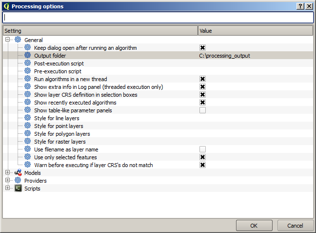
Now when you run an algorithm, just use the filename instead of the full path. For instance, with the configuration shown above, if you enter graticule.shp as the output path for the algorithm that we have just used, the result will be saved in D:\processing_output\graticule.shp. You can still enter a full path in case you want a result to be saved in a different folder.
Încercați să rulați algoritmul Creare grilă folosind diferite mărimi ale grilei, și, totodată, utilizând diverse tipuri de grilă.