16. Working with Mesh Data

16.1. What’s a mesh?

A mesh is an unstructured grid usually with temporal and other components. The spatial component contains a collection of vertices, edges and faces in 2D or 3D space:

• vertices - XY(Z) points (in the layer’s coordinate reference system)

• edges - connect pairs of vertices

• faces - a face is a set of edges forming a closed shape - typically a triangle or a quadrilateral (quad), rarely polygons with more vertices

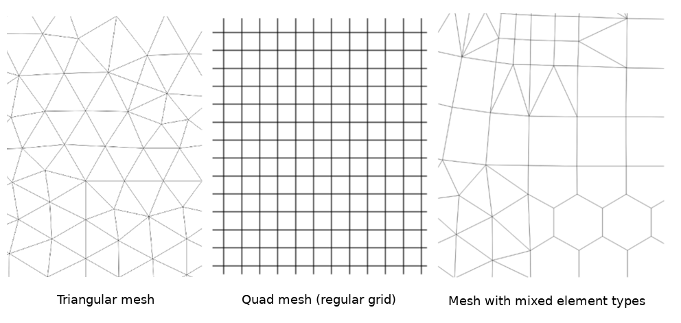
Fig. 16.1 Different mesh types

QGIS can currently render mesh data using triangles or regular quads.

Mesh provides information about the spatial structure. In addition, the mesh can have datasets (groups) that assign a value to every vertex. For example, having a triangular mesh with numbered vertices as shown in the image below:

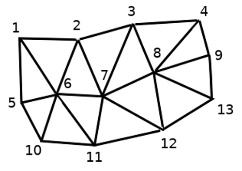
Fig. 16.2 Triangular grid with numbered vertices

Each vertex can store different datasets (typically multiple quantities), and those datasets can also have a temporal dimension. Thus, a single file may contain multiple datasets.

The following table gives an idea about the information that can be stored in mesh datasets. Table columns represent indices of mesh vertices, each row represents one dataset. Datasets can have different datatypes. In this case, it stores wind velocity at 10m at a particular moments in time (t1, t2, t3).

In a similar way, the mesh dataset can also store vector values for each vertex. For example, wind direction vector at the given time stamps:

10 metre wind	1	2	3	…
10 metre speed at time=t1	17251	24918	32858	…
10 metre speed at time=t2	19168	23001	36418	…
10 metre speed at time=t3	21085	30668	17251	…
…	…	…	…	…
10m wind direction time=t1	[20,2]	[20,3]	[20,4.5]	…
10m wind direction time=t2	[21,3]	[21,4]	[21,5.5]	…
10m wind direction time=t3	[22,4]	[22,5]	[22,6.5]	…
…	…	…	…	…

We can visualize the data by assigning colors to values (similarly to how it is done with Singleband pseudocolor raster rendering) and interpolating data between vertices according to the mesh topology. It is common that some quantities are 2D vectors rather than being simple scalar values (e.g. wind direction). For such quantities it is desirable to display arrows indicating the directions.

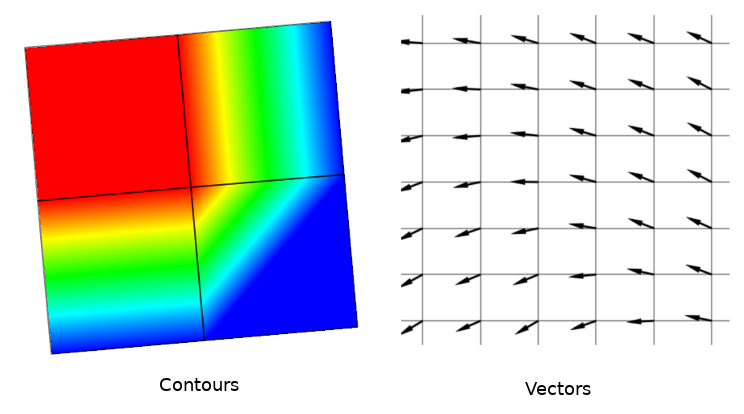
Fig. 16.3 Possible visualisation of mesh data

16.2. Supported formats

QGIS accesses mesh data using the MDAL drivers. Hence, the natively supported formats are:

• NetCDF: Generic format for scientific data

• GRIB: Format commonly used in meteorology

• XMDF: As an example, hydraulic outputs from TUFLOW modelling package

• DAT: Outputs of various hydrodynamic modelling packages (e.g. BASEMENT, HYDRO_AS-2D, TUFLOW)

• 3Di: 3Di modelling package format based on Climate and Forecast Conventions (http://cfconventions.org/)

• Some examples of mesh datasets can be found at https://apps.ecmwf.int/datasets/data/interim-full-daily/levtype=sfc/

To load a mesh dataset into QGIS, use the Mesh tab in the Data Source Manager dialog. Read Loading a mesh layer for more details.

16.3. Mesh Dataset Properties

16.3.1. Information Properties

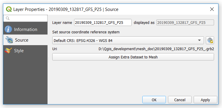
Fig. 16.4 Mesh Layer Properties

The Information tab is read-only and represents an interesting place to quickly grab summarized information and metadata on the current layer. Provided information are (based on the provider of the layer) uri, vertex count, face count and dataset groups count.

16.3.2. Source Properties

The Source tab displays basic information about the selected mesh, including:

• the Layer name to display in the Layers panel

• setting the Coordinate Reference System: Displays the layer’s Coordinate Reference System (CRS). You can change the layer’s CRS by selecting a recently used one in the drop-down list or clicking on Select CRS button (see Coordinate Reference System Selector). Use this process only if the CRS applied to the layer is wrong or if none was applied.

Use the Assign Extra Dataset to Mesh button to add more groups to the current mesh layer.

16.3.3. Symbology Properties

Click the Symbology button to activate the dialog as shown in the following image:

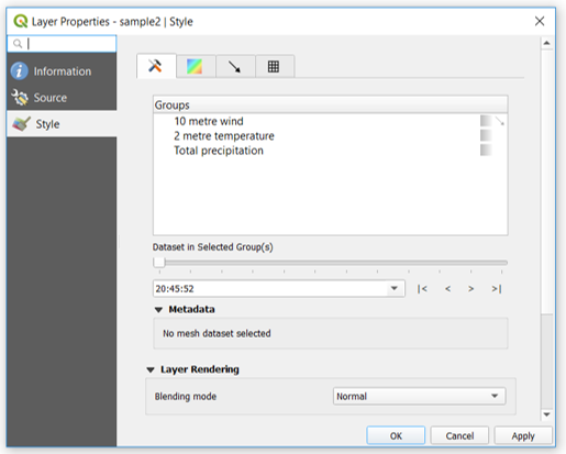
Fig. 16.5 Mesh Layer Symbology

Symbology properties are divided in several tabs:

• General

• Contours Symbology

• Vectors Symbology

• Rendering

16.3.3.1. General

The tab presents the following items:

• groups available in the mesh dataset

• dataset in the selected group(s), for example, if the layer has a temporal dimension

• metadata if available

• blending mode available for the selected dataset.

The slider , the combo box and the |<, <, >, >| buttons allow to explore another dimension of the data, if available. As the slider moves, the metadata is presented accordingly. See the figure Mesh groups below as an example. The map canvas will display the selected dataset group as well.

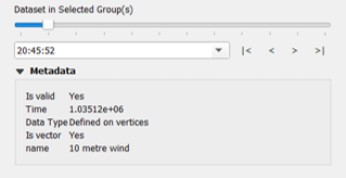
Fig. 16.6 Dataset in Selected Group(s)

You can apply symbology to each group using the tabs.

16.3.3.2. Contours Symbology

Under Groups, click on to show contours with default visualization parameters.

In the tab you can see and change the current visualization options of contours for the selected group, as shown in Fig. 16.7 below:

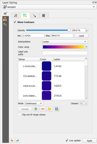
Fig. 16.7 Styling Contours in a Mesh Layer

Use the slide bar or combo box to set the opacity of the current group.

Use Load to adjust the min and max values of the current group.

The Interpolation list contains three options to render contours: Linear, Discrete and Exact.

The Color ramp widget opens the color ramp drop-down shortcut.

The Label unit suffix is a label added after the value in the legend.

By selecting Continuous in the classification Mode, QGIS creates classes automatically considering the Min and Max values. With ‘Equal interval’, you only need to select the number of classes using the combo box Classes and press the button Classify.

The button ^{Add values manually} adds a value to the individual color table. The button ^{Remove selected row} deletes a value from the individual color table. Double clicking on the value column lets you insert a specific value. Double clicking on the color column opens the dialog Change color, where you can select a color to apply on that value.

16.3.3.3. Vectors Symbology

In the tab , click on to display vectors if available. The map canvas will display the vectors in the selected group with default parameters. Click on the tab to change the visualization parameters for vectors as shown in the image below:

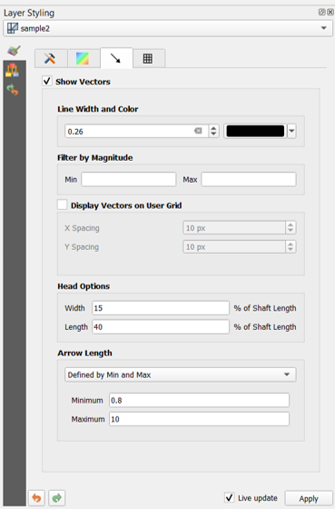
Fig. 16.8 Styling Vectors in a Mesh Layer

The line width can be set using the combo box or typing the value. The color widget opens the dialog Change color, where you can select a color to apply to vectors.

Enter values for Min and Max to filter vectors according to their magnitude.

Check on the box Display Vectors on User Grid and specify the X spacing and the Y spacing, QGIS will render the vector considering the given spacing.

With the Head Options Head Options, QGIS allows the shape of the arrow head to be set by specifying width and length (in percentage).

Vector’s Arrow length can be rendered in QGIS in three different ways:

• Defined by Min and Max: You specify the minimum and maximum length for the vectors, QGIS will adjust their visualization accordingly

• Scale to magnitude: You specify the (multiplying) factor to use

• Fixed: all the vectors are shown with the same length

16.3.3.4. Renderização

In the tab , QGIS offers two possibilities to display the grid, as shown in Fig. 16.9:

• Native Mesh Rendering that shows quadrants

• Triangular Mesh Rendering that display triangles

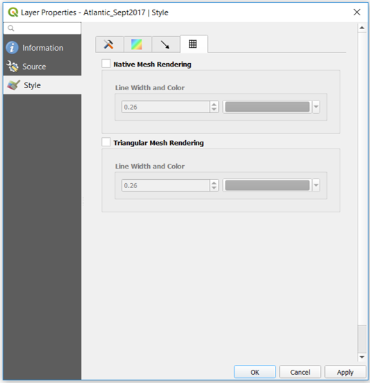
Fig. 16.9 Mesh Rendering

The line width and color can be changed in this dialog, and both the grid renderings can be turned off.