13.1. Opening Data
As part of an Open Source Software ecosystem, QGIS is built upon different libraries that, combined with its own providers, offer capabilities to read and often write a lot of formats:
Vector data formats include GeoPackage, GML, GeoJSON, GPX, KML, Comma Separated Values, ESRI formats (Shapefile, Geodatabase…), MapInfo and MicroStation file formats, AutoCAD DWG/DXF, GRASS and many more… Read the complete list of supported vector formats.
Raster data formats include GeoTIFF, JPEG, ASCII Gridded XYZ, MBTiles, R or Idrisi rasters, GDAL Virtual, SRTM, Sentinel Data, ERDAS IMAGINE, ArcInfo Binary Grid, ArcInfo ASCII Grid, and many more… Read the complete list of supported raster formats.
Database formats include PostgreSQL/PostGIS, SQLite/SpatiaLite, Oracle, DB2 or MSSQL Spatial, MySQL…
Web map and data services (WM(T)S, WFS, WCS, CSW, XYZ tiles, ArcGIS services, …) are also handled by QGIS providers. See Working with OGC / ISO protocols for more information about some of these.
You can read supported files from archived folders and use QGIS native formats such as QML files (QML - The QGIS Style File Format) and virtual and memory layers.
More than 80 vector and 140 raster formats are supported by GDAL and QGIS native providers.
Nota
Not all of the listed formats may work in QGIS for various reasons. For
example, some require external proprietary libraries, or the GDAL/OGR
installation of your OS may not have been built to support the format you
want to use. To see the list of available formats, run the command line
ogrinfo --formats (for vector) and gdalinfo --formats (for raster),
or check the menu in QGIS.
In QGIS, depending on the data format, there are different tools to open a
dataset, mainly available in the menu
or from the Manage Layers toolbar (enabled through
menu).
However, all these tools point to a unique dialog, the Data Source
Manager dialog, that you can open with the  Open Data Source Manager button, available on the Data Source
Manager Toolbar, or by pressing Ctrl+L.
The Data Source Manager dialog(Fig. 13.1) offers a unified interface to open
vector or raster file-based data as well as databases or web services supported
by QGIS.
It can be set modal or not with the
Open Data Source Manager button, available on the Data Source
Manager Toolbar, or by pressing Ctrl+L.
The Data Source Manager dialog(Fig. 13.1) offers a unified interface to open
vector or raster file-based data as well as databases or web services supported
by QGIS.
It can be set modal or not with the  Modeless data source manager dialog
in the menu.
Modeless data source manager dialog
in the menu.
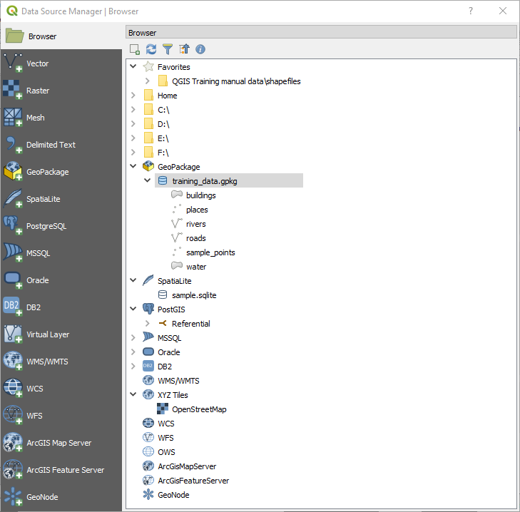
Fig. 13.1 QGIS Data Source Manager dialog
Beside this main entry point, you also have the  DB Manager plugin that offers advanced capabilities to analyze and
manipulate connected databases.
More information on DB Manager capabilities can be found in DB Manager Plugin.
DB Manager plugin that offers advanced capabilities to analyze and
manipulate connected databases.
More information on DB Manager capabilities can be found in DB Manager Plugin.
There are many other tools, native or third-party plugins, that help you open various data formats.
This chapter will describe only the tools provided by default in QGIS for loading data. It will mainly focus on the Data Source Manager dialog but more than describing each tab, it will also explore the tools based on the data provider or format specificities.
13.1.1. The Browser Panel
The Browser is one of the main ways to quickly and easily add your data to projects. It’s available as:
a Data Source Manager tab, enabled pressing the
Open Data Source Manager button (Ctrl+L);as a QGIS panel you can open from the menu (or
 ) or by pressing Ctrl+2.
In both cases, the Browser helps you navigate in your file system and manage geodata, regardless the type of layer (raster, vector, table), or the datasource format (plain or compressed files, databases, web services).
13.1.1.1. Exploring the Interface
At the top of the Browser panel, you find some buttons that help you to:
 Add Selected Layers: you can also add data to the map
canvas by selecting Add selected layer(s) from the layer’s context menu;
Add Selected Layers: you can also add data to the map
canvas by selecting Add selected layer(s) from the layer’s context menu; Refresh the browser tree;
 Filter Browser to search for specific data. Enter a search
word or wildcard and the browser will filter the tree to only show paths to
matching DB tables, filenames or folders – other data or folders won’t be
displayed. See the Browser Panel(2) example in Fig. 13.2.
The comparison can be case-sensitive or not. It can also be set to:
Filter Browser to search for specific data. Enter a search
word or wildcard and the browser will filter the tree to only show paths to
matching DB tables, filenames or folders – other data or folders won’t be
displayed. See the Browser Panel(2) example in Fig. 13.2.
The comparison can be case-sensitive or not. It can also be set to:Normal: show items containing the search text
Wildcard(s): fine tune the search using the
?and/or*characters to specify the position of the search textRegular expression
 Collapse All the whole tree;
 Enable/disable properties widget: when toggled on,
a new widget is added at the bottom of the panel showing, if applicable,
metadata for the selected item.
Enable/disable properties widget: when toggled on,
a new widget is added at the bottom of the panel showing, if applicable,
metadata for the selected item.
The entries in the Browser panel are organised hierarchically, and there are several top level entries:
Favorites where you can place shortcuts to often used locations
Spatial Bookmarks where you can store often used map extents (see Marcadores Espaciais)
Project Home: for a quick access to the folder in which (most of) the data related to your project are stored. The default value is the directory where your project file resides.
Home directory in the file system and the filesystem root directory.
Connected local or network drives
Then comes a number of container / database types and service protocols, depending on your platform and underlying libraries:
 GeoPackage
 SpatiaLite
 PostGIS
 MSSQL
MSSQL Oracle
 DB2
DB2 WMS/WMTS
 Vector Tiles
 XYZ Tiles
 WCS
WCS WFS/OGC API-Features
 OWS
OWS ArcGIS Map Service
 ArcGIS Feature Service
 GeoNode
13.1.1.2. Interacting with the Browser items
The browser supports drag and drop within the browser, from the browser to the canvas and Layers panel, and from the Layers panel to layer containers (e.g. GeoPackage) in the browser.
Project file items inside the browser can be expanded, showing the full layer tree (including groups) contained within that project. Project items are treated the same way as any other item in the browser, so they can be dragged and dropped within the browser (for example to copy a layer item to a geopackage file) or added to the current project through drag and drop or double click.
The context menu for an element in the Browser panel is opened by right-clicking on it.
For file system directory entries, the context menu offers the following:
to create in the selected entry a:
Directory…
GeoPackage…
ShapeFile…
Add as a Favorite: favorite folders can be renamed (Rename favorite…) or removed (Remove favorite) any time.
Hide from Browser: hidden folders can be toggled to visible from the setting
Fast Scan this Directory
Open Directory
Open in Terminal
Propriedades…
Directory Properties…
For leaf entries that can act as layers in the project, the context menu will have supporting entries. For example, for non-database, non-service-based vector, raster and mesh data sources:
Delete File «<name of file>»…
Export Layer –> To File…
Add Layer to Project
Layer Properties
File Properties
In the Layer properties entry, you will find (similar to what you will find in the vector and raster layer properties once the layers have been added to the project):
Metadata for the layer. Metadata groups: Information from provider (if possible, Path will be a hyperlink to the source), Identification, Extent, Access, Fields (for vector layers), Bands (for raster layers), Contacts, Links (for vector layers), References (for raster layers), History.
A Preview panel
The attribute table for vector sources (in the Attributes panel).
To add a layer to the project using the Browser:
Enable the Browser as described above. A browser tree with your file system, databases and web services is displayed. You may need to connect databases and web services before they appear (see dedicated sections).
Find the layer in the list.
Use the context menu, double-click its name, or drag-and-drop it into the map canvas. Your layer is now added to the Layers panel and can be viewed on the map canvas.
Dica
Open a QGIS project directly from the browser
You can also open a QGIS project directly from the Browser panel by double-clicking its name or by drag-and-drop into the map canvas.
Once a file is loaded, you can zoom around it using the map navigation tools. To change the style of a layer, open the Layer Properties dialog by double-clicking on the layer name or by right-clicking on the name in the legend and choosing from the context menu. See section Symbology Properties for more information on setting symbology for vector layers.
Right-clicking an item in the browser tree helps you to:
for a file or a table, display its metadata or open it in your project. Tables can even be renamed, deleted or truncated.
for a folder, bookmark it into your favourites or hide it from the browser tree. Hidden folders can be managed from the tab.
manage your spatial bookmarks: bookmarks can be created, exported and imported as
XMLfiles.create a connection to a database or a web service.
refresh, rename or delete a schema.
You can also import files into databases or copy tables from one schema/database to another with a simple drag-and-drop. There is a second browser panel available to avoid long scrolling while dragging. Just select the file and drag-and-drop from one panel to the other.
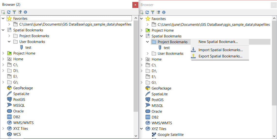
Fig. 13.2 QGIS Browser panels side-by-side
Dica
Add layers to QGIS by simple drag-and-drop from your OS file browser
You can also add file(s) to the project by drag-and-dropping them from your operating system file browser to the Layers Panel or the map canvas.
13.1.2. The DB Manager
The DB Manager Plugin is another tool for integrating and managing spatial database formats supported by QGIS (PostGIS, SpatiaLite, GeoPackage, Oracle Spatial, MSSQL, DB2, Virtual layers). It can be activated from the menu.
The DB Manager Plugin provides several features:
connect to databases and display their structure and contents
preview tables of databases
add layers to the map canvas, either by double-clicking or drag-and-drop.
add layers to a database from the QGIS Browser or from another database
create SQL queries and add their output to the map canvas
create virtual layers
More information on DB Manager capabilities is found in DB Manager Plugin.
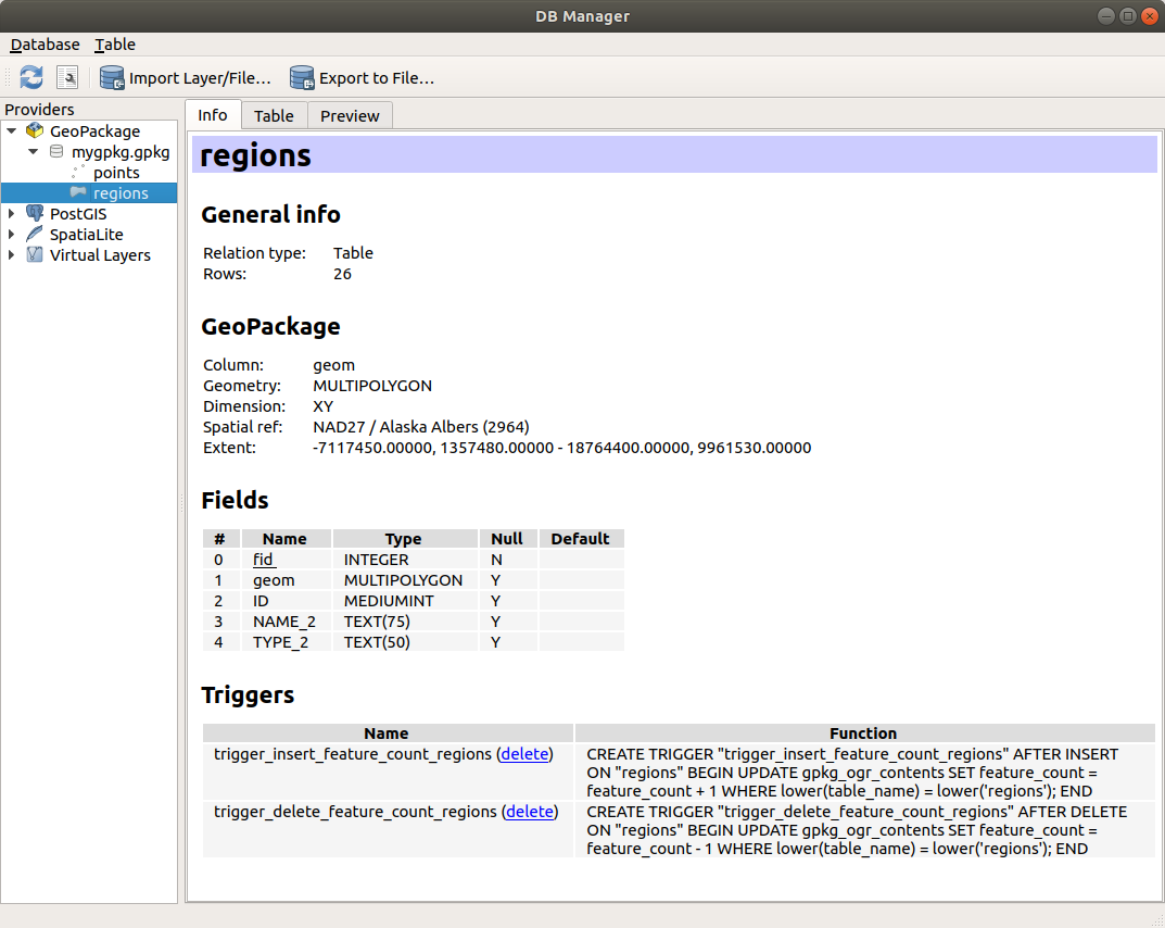
Fig. 13.3 DB Manager dialog
13.1.3. Provider-based loading tools
Beside the Browser Panel and the DB Manager, the main tools provided by QGIS to add layers, you’ll also find tools that are specific to data providers.
Nota
Some external plugins also provide tools to open specific format files in QGIS.
13.1.3.1. Loading a layer from a file
To load a layer from a file:
Open the layer type tab in the Data Source Manager dialog, ie click the
Open Data Source Manager
button (or press Ctrl+L) and enable the target tab or:for vector data (like GML, ESRI Shapefile, Mapinfo and DXF layers): press Ctrl+Shift+V, select the
 Add Vector Layer menu option or
click on the Add Vector Layer toolbar button.
Add Vector Layer menu option or
click on the Add Vector Layer toolbar button.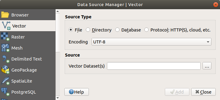
Fig. 13.4 Add Vector Layer Dialog
for raster data (like GeoTiff, MBTiles, GRIdded Binary and DWG layers): press Ctrl+Shift+R, select the
 Add Raster Layer menu option or
click on the Add Raster Layer toolbar button.
Add Raster Layer menu option or
click on the Add Raster Layer toolbar button.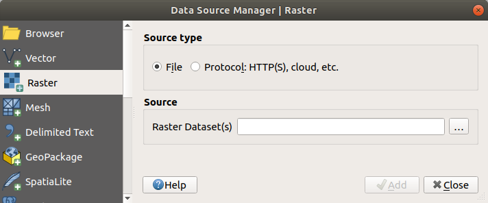
Fig. 13.5 Add Raster Layer Dialog
Check
 File source type
Click on the … Browse button
Navigate the file system and load a supported data source. More than one layer can be loaded at the same time by holding down the Ctrl key and clicking on multiple items in the dialog or holding down the Shift key to select a range of items by clicking on the first and last items in the range. Only formats that have been well tested appear in the formats filter. Other formats can be loaded by selecting
All files(the top item in the pull-down menu).Press Open to load the selected file into Data Source Manager dialog
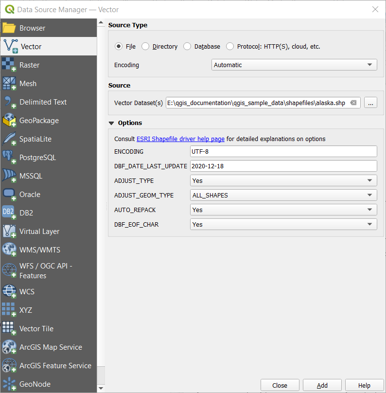
Fig. 13.6 Loading a Shapefile with open options
Press Add to load the file in QGIS and display them in the map view. Fig. 13.7 shows QGIS after loading the
alaska.shpfile.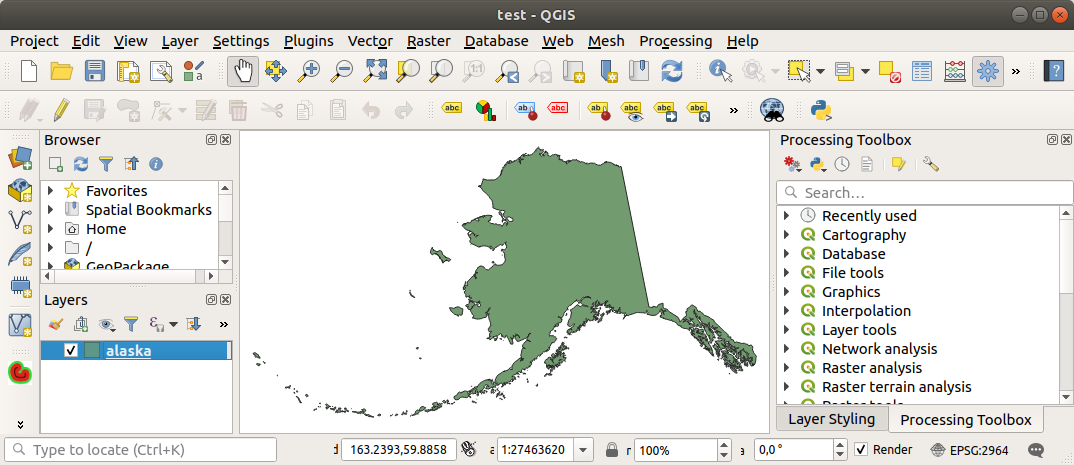
Fig. 13.7 QGIS with Shapefile of Alaska loaded
Nota
For loading vector files the GDAL driver offers to define open actions. These will be shown when the vector file is selected. Options are described in detail on https://gdal.org/drivers/vector/ .
Nota
Because some formats like MapInfo (e.g., .tab) or Autocad (.dxf)
allow mixing different types of geometry in a single file, loading such
datasets opens a dialog to select geometries to use in order to have one
geometry per layer.
The Add Vector Layer and Add Raster
Layer tabs allow loading of layers from source types other than File:
You can load specific vector formats like
ArcInfo Binary Coverage,UK. National Transfer Format, as well as the raw TIGER format of theUS Census BureauorOpenfileGDB. To do that, you select Directory as Source type.
In this case, a directory can be selected in the dialog after pressing
… Browse.With the
Database source type you can select an
existing database connection or create one to the selected database type.
Some possible database types are ODBC,Esri Personal Geodatabase,MSSQLas well asPostgreSQLorMySQL.Pressing the New button opens the Create a New OGR Database Connection dialog whose parameters are among the ones you can find in Creating a stored Connection. Pressing Open lets you select from the available tables, for example of PostGIS enabled databases.
The
Protocol: HTTP(S), cloud, etc. source type
opens data stored locally or on the network, either publicly accessible,
or in private buckets of commercial cloud storage services.
Supported protocol types are:HTTP/HTTPS/FTP, with a URI and, if required, an authentication.Cloud storage such as
AWS S3,Google Cloud Storage,Microsoft Azure Blob,Alibaba OSS Cloud,Open Stack Swift Storage. You need to fill in the Bucket or container and the Object key.service supporting OGC
WFS 3(still experimental), usingGeoJSONorGEOJSON - Newline Delimitedformat or based onCouchDBdatabase. A URI is required, with optional authentication.For all vector source types it is possible to define the Encoding or to use the setting.
13.1.3.2. Loading a mesh layer
A mesh is an unstructured grid usually with temporal and other components. The spatial component contains a collection of vertices, edges and faces in 2D or 3D space. More information on mesh layers at Working with Mesh Data.
To add a mesh layer to QGIS:
Open the dialog, either by selecting it from the menu or clicking the
Open Data Source Manager button.Enable the
 Mesh tab on the left panel
Press the … Browse button to select the file. Various formats are supported.
Select the layer and press Add. The layer will be added using the native mesh rendering.
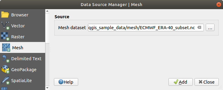
Fig. 13.8 Mesh tab in Data Source Manager
13.1.3.3. Importing a delimited text file
Delimited text files (e.g. .txt, .csv, .dat,
.wkt) can be loaded using the tools described above.
This way, they will show up as simple tables.
Sometimes, delimited text files can contain coordinates / geometries
that you could want to visualize.
This is what  Add Delimited Text Layer
is designed for.
Add Delimited Text Layer
is designed for.
Click the
Open Data Source Manager icon to
open the Data Source Manager dialogEnable the
Delimited Text tabSelect the delimited text file to import (e.g.,
qgis_sample_data/csv/elevp.csv) by clicking on the … Browse button.In the Layer name field, provide the name to use for the layer in the project (e.g.
Elevation).Configure the settings to meet your dataset and needs, as explained below.
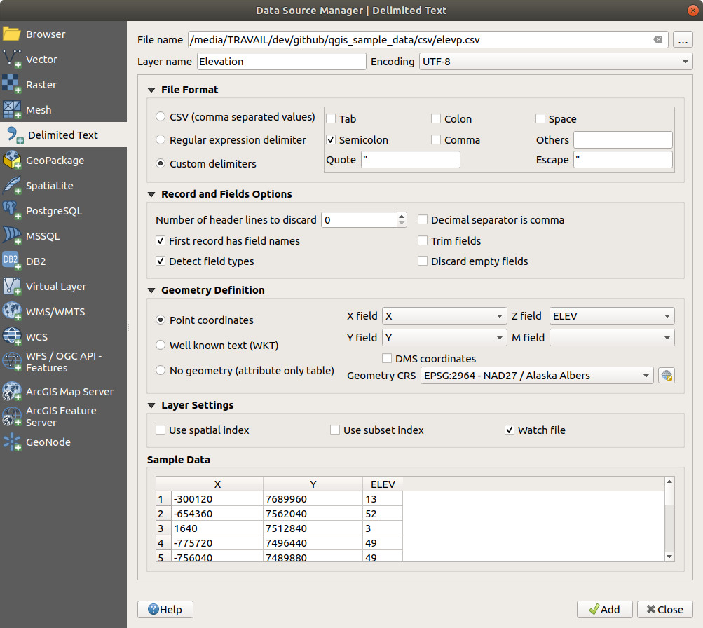
Fig. 13.9 Delimited Text Dialog
File format
Once the file is selected, QGIS attempts to parse the file with the most recently used delimiter, identifying fields and rows. To enable QGIS to correctly parse the file, it is important to select the right delimiter. You can specify a delimiter by choosing between:
- CSV (comma separated values) to use the
comma character.
 Regular expression delimiter and enter text
into the Expression field.
For example, to change the delimiter to tab, use
Regular expression delimiter and enter text
into the Expression field.
For example, to change the delimiter to tab, use \t(this is used in regular expressions for the tab character).- Custom delimiters, choosing among some predefined
delimiters like
comma,space,tab,semicolon, … .
Records and fields
Some other convenient options can be used for data recognition:
Number of header lines to discard: convenient when you want to avoid the first lines in the file in the import, either because those are blank lines or with another formatting.
- First record has field names: values in the first
line are used as field names, otherwise QGIS uses the field names
field_1,field_2… - Detect field types: automatically recognizes the field
type. If unchecked then all attributes are treated as text fields.
- Decimal separator is comma: you can force
decimal separator to be a comma.
- Trim fields: allows you to trim leading and trailing
spaces from fields.
- Discard empty fields.
As you set the parser properties, a sample data preview updates at the bottom of the dialog.
Geometry definition
Once the file is parsed, set Geometry definition to
- Point coordinates and provide the X
field, Y field, Z field (for 3-dimensional data)
and M field (for the measurement dimension) if the layer is of
point geometry type and contains such fields. If the coordinates
are defined as degrees/minutes/seconds, activate the
DMS coordinates checkbox.
Provide the appropriate Geometry CRS using the
 Select CRS widget.
 - Well known text (WKT) option if the spatial
information is represented as WKT: select the Geometry field
containing the WKT geometry and choose the approriate Geometry
field or let QGIS auto-detect it.
Provide the appropriate Geometry CRS using the
Select CRS widget.
If the file contains non-spatial data, activate
No
geometry (attribute only table) and it will be loaded as an ordinary table.
Layer settings
Additionally, you can enable:
- Use spatial index to improve the performance of
displaying and spatially selecting features.
- Use subset index to improve performance of subset
filters (when defined in the layer properties).
- Watch file to watch for changes to the file by other
applications while QGIS is running.
At the end, click Add to add the layer to the map.
In our example, a point layer named Elevation is added to the project
and behaves like any other map layer in QGIS.
This layer is the result of a query on the .csv source file
(hence, linked to it) and would require
to be saved in order to get a spatial layer on disk.
13.1.3.4. Importing a DXF or DWG file
DXF and DWG files can be added to QGIS by simple drag-and-drop
from the Browser Panel.
You will be prompted to select the sublayers you would like to add
to the project. Layers are added with random style properties.
Nota
For DXF files containing several geometry types (point, line and/or polygon), the name of the layers will be generated as <filename.dxf> entities <geometry type>.
To keep the dxf/dwg file structure and its symbology in QGIS, you may want to use the dedicated tool which allows you to:
import elements from the drawing file into a GeoPackage database.
add imported elements to the project.
In the DWG/DXF Import dialog, to import the drawing file contents:
Input the location of the Target package, i.e. the new GeoPackage file that will store the data. If an existing file is provided, then it will be overwritten.
Specify the coordinate reference system of the data in the drawing file.
Check
Expand block references to import the
blocks in the drawing file as normal elements.Check
Use curves to promote the imported layers
to a curvedgeometry type.Use the Import button to select the DWG/DXF file to use (one per geopackage). The GeoPackage database will be automatically populated with the drawing file content. Depending on the size of the file, this can take some time.
After the .dwg or .dxf data has been imported into the
GeoPackage database, the frame in the lower half of the dialog is
populated with the list of layers from the imported file.
There you can select which layers to add to the QGIS project:
At the top, set a Group name to group the drawing files in the project.
Check layers to show: Each selected layer is added to an ad hoc group which contains vector layers for the point, line, label and area features of the drawing layer. The style of the layers will resemble the look they originally had in *CAD.
Choose if the layer should be visible at opening.
Checking the
Merge layers option places all
layers in a single group.Press OK to open the layers in QGIS.
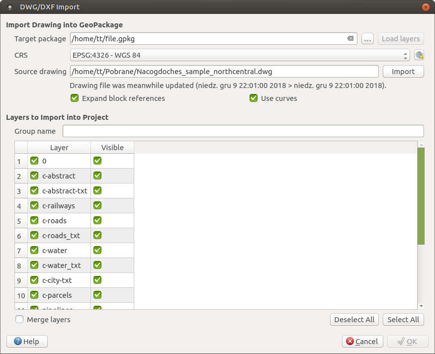
Fig. 13.10 Import dialog for DWG/DXF files
13.1.3.5. Importing OpenStreetMap Vectors
The OpenStreetMap project is popular because in many countries no free geodata such as digital road maps are available. The objective of the OSM project is to create a free editable map of the world from GPS data, aerial photography and local knowledge. To support this objective, QGIS provides support for OSM data.
Using the Browser Panel, you can load an .osm file to the
map canvas, in which case you’ll get a dialog to select sublayers based on the
geometry type.
The loaded layers will contain all the data of that geometry type
in the .osm file, and keep the osm file data structure.
13.1.3.6. SpatiaLite Layers
 The first time you load data from a SpatiaLite
database, begin by:
The first time you load data from a SpatiaLite
database, begin by:
clicking on the
Add SpatiaLite Layer toolbar
buttonselecting the
option from the menuor by typing Ctrl+Shift+L
This will bring up a window that will allow you either to connect to a
SpatiaLite database already known to QGIS (which you choose from the
drop-down menu) or to define a new connection to a new database. To define a
new connection, click on New and use the file browser to point to
your SpatiaLite database, which is a file with a .sqlite extension.
QGIS also supports editable views in SpatiaLite.
13.1.3.7. GPS
Loading GPS data in QGIS can be done using the core plugin GPS Tools.
Instructions are found in section Módulo GPS.
13.1.3.8. GRASS
Working with GRASS vector data is described in section Integração GRASS SIG.
13.1.3.9. Database related tools
Creating a stored Connection
In order to read and write tables from a database format QGIS supports you have to create a connection to that database. While QGIS Browser Panel is the simplest and recommanded way to connect to and use databases, QGIS provides other tools to connect to each of them and load their tables:
 or by typing
Ctrl+Shift+D
or by typing
Ctrl+Shift+D
 or by typing
Ctrl+Shift+O
or by typing
Ctrl+Shift+O or by typing
Ctrl+Shift+2
or by typing
Ctrl+Shift+2
These tools are accessible either from the Manage Layers Toolbar and the menu. Connecting to SpatiaLite database is described at SpatiaLite Layers.
Dica
Create connection to database from the QGIS Browser Panel
Selecting the corresponding database format in the Browser tree, right-clicking and choosing connect will provide you with the database connection dialog.
Most of the connection dialogs follow a common basis that will be described below using the PostgreSQL database tool as an example. For additional settings specific to other providers, you can find corresponding descriptions at:
The first time you use a PostGIS data source, you must create a connection to a database that contains the data. Begin by clicking the appropriate button as exposed above, opening an Add PostGIS Table(s) dialog (see Fig. 13.12). To access the connection manager, click on the New button to display the Create a New PostGIS Connection dialog.
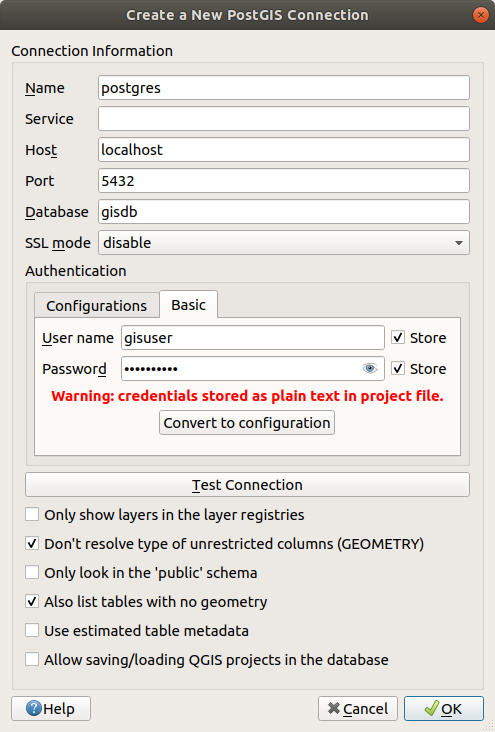
Fig. 13.11 Create a New PostGIS Connection Dialog
The parameters required for a PostGIS connection are explained below. For the other database types, see their differences at Particular Connection requirements.
Name: A name for this connection. It can be the same as Database.
Service: Service parameter to be used alternatively to hostname/port (and potentially database). This can be defined in
pg_service.conf. Check the PostgreSQL Service connection file section for more details.Host: Name of the database host. This must be a resolvable host name such as would be used to open a TCP/IP connection or ping the host. If the database is on the same computer as QGIS, simply enter localhost here.
Port: Port number the PostgreSQL database server listens on. The default port for PostGIS is
5432.Database: Name of the database.
SSL mode: SSL encryption setup The following options are available:
Prefer (the default): I don’t care about encryption, but I wish to pay the overhead of encryption if the server supports it.
Require: I want my data to be encrypted, and I accept the overhead. I trust that the network will make sure I always connect to the server I want.
Verify CA: I want my data encrypted, and I accept the overhead. I want to be sure that I connect to a server that I trust.
Verify Full: I want my data encrypted, and I accept the overhead. I want to be sure that I connect to a server I trust, and that it’s the one I specify.
Allow: I don’t care about security, but I will pay the overhead of encryption if the server insists on it.
Disable: I don’t care about security, and I don’t want to pay the overhead of encryption.
Authentication, basic.
User name: User name used to log in to the database.
Password: Password used with Username to connect to the database.
You can save any or both of the
User nameandPasswordparameters, in which case they will be used by default each time you need to connect to this database. If not saved, you’ll be prompted to supply the credentials to connect to the database in next QGIS sessions. The connection parameters you entered are stored in a temporary internal cache and returned whenever a username/password for the same database is requested, until you end the current QGIS session.Aviso
QGIS User Settings and Security
In the Authentication tab, saving username and password will keep unprotected credentials in the connection configuration. Those credentials will be visible if, for instance, you share the project file with someone. Therefore, it is advisable to save your credentials in an Authentication configuration instead (Configurations tab - See Sistema de Autenticação for more details) or in a service connection file (see PostgreSQL Service connection file for example).
Authentication, configurations. Choose an authentication configuration. You can add configurations using the
 button. Choices are:
Basic authentication
PKI PKCS#12 authentication
PKI paths authentication
PKI stored identity certificate
Optionally, depending on the type of database, you can activate the following checkboxes:
- Only show layers in the layer registries
- Don’t resolve type of unrestricted columns (GEOMETRY)
- Only look in the “public” schema
- Also list tables with no geometry
- Use estimated table metadata
- Allow saving/loading QGIS projects in the database
- more details here
Dica
Use estimated table metadata to speed up operations
When initializing layers, various queries may be needed to establish the characteristics of the geometries stored in the database table. When the Use estimated table metadata option is checked, these queries examine only a sample of the rows and use the table statistics, rather than the entire table. This can drastically speed up operations on large datasets, but may result in incorrect characterization of layers (e.g. the feature count of filtered layers will not be accurately determined) and may even cause strange behaviour if columns that are supposed to be unique actually are not.
Once all parameters and options are set, you can test the connection by clicking the Test Connection button or apply it by clicking the OK button. From Add PostGIS Table(s), click now on Connect, and the dialog is filled with tables from the selected database (as shown in Fig. 13.12).
Particular Connection requirements
Because of database type particularities, provided options are not the same. Database specific options are described below.
PostgreSQL Service connection file
The service connection file allows PostgreSQL connection parameters to be associated with a single service name. That service name can then be specified by a client and the associated settings will be used.
It’s called .pg_service.conf under *nix systems (GNU/Linux,
macOS etc.) and pg_service.conf on Windows.
The service file can look like this:
[water_service]
host=192.168.0.45
port=5433
dbname=gisdb
user=paul
password=paulspass

[wastewater_service]
host=dbserver.com
dbname=water
user=waterpass
Nota
There are two services in the above example: water_service
and wastewater_service. You can use these to connect from QGIS,
pgAdmin, etc. by specifying only the name of the service you want to
connect to (without the enclosing brackets).
If you want to use the service with psql you need to do something
like export PGSERVICE=water_service before doing your psql commands.
You can find all the PostgreSQL parameters here
Nota
If you don’t want to save the passwords in the service file you can use the .pg_pass option.
On *nix operating systems (GNU/Linux, macOS etc.) you can save the
.pg_service.conf file in the user’s home directory and
PostgreSQL clients will automatically be aware of it.
For example, if the logged user is web, .pg_service.conf should
be saved in the /home/web/ directory in order to directly work (without
specifying any other environment variables).
You can specify the location of the service file by creating a
PGSERVICEFILE environment variable (e.g. run the
export PGSERVICEFILE=/home/web/.pg_service.conf
command under your *nix OS to temporarily set the PGSERVICEFILE
variable)
You can also make the service file available system-wide (all users) either by
placing the .pg_service.conf file in pg_config --sysconfdir or by
adding the PGSYSCONFDIR environment variable to specify the directory
containing the service file. If service definitions with the same name exist
in the user and the system file, the user file takes precedence.
Aviso
There are some caveats under Windows:
The service file should be saved as
pg_service.confand not as.pg_service.conf.The service file should be saved in Unix format in order to work. One way to do it is to open it with Notepad++ and .
You can add environmental variables in various ways; a tested one, known to work reliably, is adding
PGSERVICEFILEwith the path - e.g.C:\Users\John\pg_service.confAfter adding an environment variable you may also need to restart the computer.
Connecting to Oracle Spatial
The spatial features in Oracle Spatial aid users in managing geographic and location data in a native type within an Oracle database. In addition to some of the options in Creating a stored Connection, the connection dialog proposes:
Database: SID or SERVICE_NAME of the Oracle instance;
Port: Port number the Oracle database server listens on. The default port is
1521;Options: Oracle connection specific options (e.g. OCI_ATTR_PREFETCH_ROWS, OCI_ATTR_PREFETCH_MEMORY). The format of the options string is a semicolon separated list of option names or option=value pairs;
Workspace: Workspace to switch to;
Schema: Schema in which the data are stored
Optionally, you can activate the following checkboxes:
- Only look in metadata table: restricts the displayed
tables to those that are in the
all_sdo_geom_metadataview. This can speed up the initial display of spatial tables. - Only look for user’s tables: when searching for spatial
tables, restricts the search to tables that are owned by the user.
- Also list tables with no geometry: indicates that
tables without geometry should also be listed by default.
- Use estimated table statistics for the layer metadata:
when the layer is set up, various metadata are required for the Oracle table.
This includes information such as the table row count, geometry type and
spatial extents of the data in the geometry column. If the table contains a
large number of rows, determining this metadata can be time-consuming. By
activating this option, the following fast table metadata operations are
done: Row count is determined from
all_tables.num_rows. Table extents are always determined with the SDO_TUNE.EXTENTS_OF function, even if a layer filter is applied. Table geometry is determined from the first 100 non-null geometry rows in the table. - Only existing geometry types: only lists the existing
geometry types and don’t offer to add others.
- Include additional geometry attributes.
Dica
Oracle Spatial Layers
Normally, an Oracle Spatial layer is defined by an entry in the USER_SDO_METADATA table.
To ensure that selection tools work correctly, it is recommended that your tables have a primary key.
Connecting to DB2 Spatial
In addition to some of the options described in Creating a stored Connection, the connection to a DB2 database (see DB2 Spatial Layers for more information) can be specified using either a Service/DSN name defined to ODBC or Driver, Host and Port.
An ODBC Service/DSN connection requires the service name defined to ODBC.
A driver/host/port connection requires:
Driver: Name of the DB2 driver. Typically this would be IBM DB2 ODBC DRIVER.
DB2 Host: Name of the database host. This must be a resolvable host name such as would be used to open a TCP/IP connection or ping the host. If the database is on the same computer as QGIS, simply enter localhost here.
DB2 Port: Port number the DB2 database server listens on. The default DB2 LUW port is
50000. The default DB2 z/OS port is446.
Dica
DB2 Spatial Layers
A DB2 Spatial layer is defined by a row in the DB2GSE.ST_GEOMETRY_COLUMNS view.
Nota
In order to work effectively with DB2 spatial tables in QGIS, it is important that tables have an INTEGER or BIGINT column defined as PRIMARY KEY and if new features are going to be added, this column should also have the GENERATED characteristic.
It is also helpful for the spatial column to be registered with a specific
spatial reference identifier (most often 4326 for WGS84 coordinates).
A spatial column can be registered by calling the
ST_Register_Spatial_Column stored procedure.
Connecting to MSSQL Spatial
In addition to some of the options in Creating a stored Connection, creating a new MSSQL connection dialog proposes you to fill a Provider/DSN name. You can also display available databases.
Loading a Database Layer
Once you have one or more connections defined to a database (see section Creating a stored Connection), you can load layers from it. Of course, this requires that data are available. See section Importing Data into PostgreSQL for a discussion on importing data into a PostGIS database.
To load a layer from a database, you can perform the following steps:
Open the «Add <database> table(s)» dialog (see Creating a stored Connection).
Choose the connection from the drop-down list and click Connect.
Select or unselect
Also list tables with no geometry.Optionally, use some
Search Options to reduce the
list of tables to those matching your search. You can also set this option
before you hit the Connect button, speeding up the database
fetching.Find the layer(s) you wish to add in the list of available layers.
Select it by clicking on it. You can select multiple layers by holding down the Shift or Ctrl key while clicking.
If applicable, use the Set Filter button (or double-click the layer) to start the Query Builder dialog (see section Query Builder) and define which features to load from the selected layer. The filter expression appears in the
sqlcolumn. This restriction can be removed or edited in the frame.The checkbox in the
Select at idcolumn that is activated by default gets the feature ids without the attributes and generally speeds up the data loading.Click on the Add button to add the layer to the map.
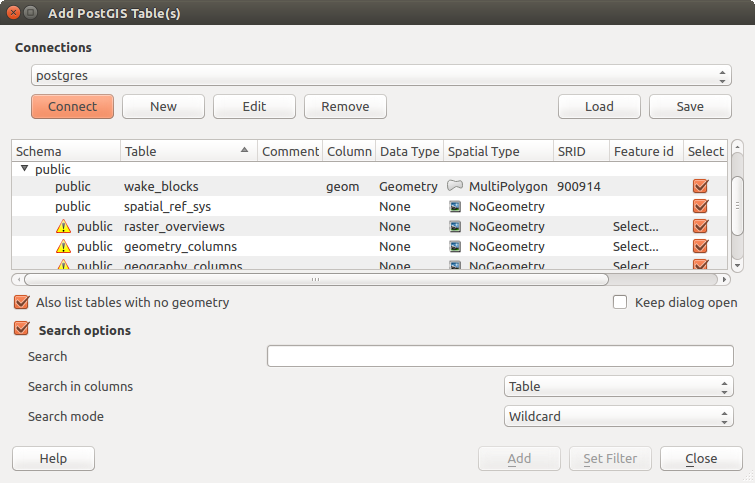
Fig. 13.12 Add PostGIS Table(s) Dialog
Dica
Use the Browser Panel to speed up loading of database table(s)
Adding DB tables from the Data Source Manager may sometimes be time consuming as QGIS fetches statistics and properties (e.g. geometry type and field, CRS, number of features) for each table beforehand. To avoid this, once the connection is set, it is better to use the Browser Panel or the DB Manager to drag and drop the database tables into the map canvas.
13.1.4. QGIS Custom formats
QGIS proposes two custom formats:
Temporary Scratch Layer: a memory layer that is bound to the project (see Creating a new Temporary Scratch Layer for more information)
Virtual Layers: a layer resulting from a query on other layer(s) (see Creating virtual layers for more information)
13.1.5. QLR - QGIS Layer Definition File
Layer definitions can be saved as a
Layer Definition File (QLR -
.qlr) using
in the layer
context menu.
The QLR format makes it possible to share «complete» QGIS layers with other QGIS users. QLR files contain links to the data sources and all the QGIS style information necessary to style the layer.
QLR files are shown in the Browser Panel and can be used to add layers (with their saved styles) to the Layers Panel. You can also drag and drop QLR files from the system file manager into the map canvas.
13.1.6. Connecting to web services
With QGIS you can get access to different types of OGC web services (WM(T)S, WFS(-T), WCS, CSW, …). Thanks to QGIS Server, you can also publish such services. Manual do utilizador QGIS Server contains descriptions of these capabilities.
13.1.6.1. Using Vector Tiles services
Vector Tiles services can be found in the Vector Tiles
top level entry in the Browser.
You can add a service by opening the context menu with a right-click
and choosing New Generic Connection ….
You set up a service by adding a Name and a URL.
The Vector Tiles Service must provide tiles in .pbf format.
The dialog provides two menus to define the
Min. Zoom Level and the
Max. Zoom Level. Vector Tiles have a
pyramid structure. By using these options you have the opportunity
to individually generate layers from the tile pyramid. These layers
will then be used to render the Vector Tile in QGIS.
For Mercator projection (used by OpenStreetMap Vector Tiles) Zoom Level 0
represents the whole world at a scale of 1:500.000.000. Zoom Level 14
represents the scale 1:35.000.
Fig. 13.13 shows the dialog with the
MapTiler planet Vector Tiles service configuration.
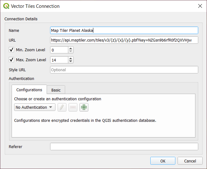
Fig. 13.13 Vector Tiles - Maptiler Planet configuration
By using New ArcGIS Vector Tile Service Connection … you can connect to ArcGIS Vector Tile Services.
13.1.6.2. Using XYZ Tile services
XYZ Tile services can be found in the XYZ Tiles top level entry in the Browser. By default, the OpenStreetMap XYZ Tile service is configured. You can add other services that use the XYZ Tile protocol by choosing New Connection in the XYZ Tiles context menu (right-click to open). Fig. 13.14 shows the dialog with the OpenStreetMap XYZ Tile service configuration.
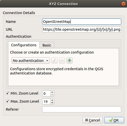
Fig. 13.14 XYZ Tiles - OpenStreetMap configuration
Configurations can be saved (Save Connections) to XML and loaded (Load Connections) through the context menu. Authentication configuration is supported. The XML file for OpenStreetMap looks like this:
<!DOCTYPE connections>
<qgsXYZTilesConnections version="1.0">
  <xyztiles url="https://tile.openstreetmap.org/{z}/{x}/{y}.png"
   zmin="0" zmax="19" tilePixelRatio="0" password="" name="OpenStreetMap"
   username="" authcfg="" referer=""/>
</qgsXYZTilesConnections>
Once a connection to a XYZ tile service is set, right-click over the entry to:
Edit… the XYZ connection settings
Delete the connection
Add layer to project: a double-click also adds the layer
View the Layer Properties… and get access to metadata and a preview of the data provided by the service. More settings are available when the layer has been loaded into the project.
Examples of XYZ Tile services:
OpenStreetMap Monochrome: URL:
http://tiles.wmflabs.org/bw-mapnik/{z}/{x}/{y}.png, Min. Zoom Level: 0, Max. Zoom Level: 19.Google Maps: URL:
https://mt1.google.com/vt/lyrs=m&x={x}&y={y}&z={z}, Min. Zoom Level: 0, Max. Zoom Level: 19.Open Weather Map Temperature: URL:
http://tile.openweathermap.org/map/temp_new/{z}/{x}/{y}.png?appid={api_key}Min. Zoom Level: 0, Max. Zoom Level: 19.