23.1.10. Raster terrain analysis
23.1.10.1. Aspect
Calculates the aspect of the Digital Terrain Model in input. The final aspect raster layer contains values from 0 to 360 that express the slope direction, starting from north (0°) and continuing clockwise.

Fig. 23.8 Aspect values
The following picture shows the aspect layer reclassified with a color ramp:

Fig. 23.9 Aspect layer reclassified
23.1.10.1.1. Parameters
Label |
Name |
Type |
Description |
|---|---|---|---|
Elevation layer |
|
[raster] |
Digital Terrain Model raster layer |
Z factor |
|
[number] Default: 1.0 |
Vertical exaggeration. This parameter is useful when the Z units differ from the X and Y units, for example feet and meters. You can use this parameter to adjust for this. The default is 1 (no exaggeration). |
Aspect |
|
[raster] |
Specify the output aspect raster layer. One of:
The file encoding can also be changed here. |
23.1.10.1.2. Outputs
Label |
Name |
Type |
Description |
|---|---|---|---|
Aspect |
|
[raster] |
The output aspect raster layer |
23.1.10.1.3. Python code
Algorithm ID: qgis:aspect
import processing
processing.run("algorithm_id", {parameter_dictionary})
The algorithm id is displayed when you hover over the algorithm in the Processing Toolbox. The parameter dictionary provides the parameter NAMEs and values. See Using processing algorithms from the console for details on how to run processing algorithms from the Python console.
23.1.10.2. Hillshade
Calculates the hillshade raster layer given an input Digital Terrain Model.
The shading of the layer is calculated according to the sun position: you have the options to change both the horizontal angle (azimuth) and the vertical angle (sun elevation) of the sun.
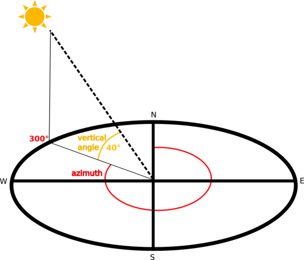
Fig. 23.10 Azimuth and vertical angle
The hillshade layer contains values from 0 (complete shadow) to 255 (complete sun). Hillshade is used usually to better understand the relief of the area.
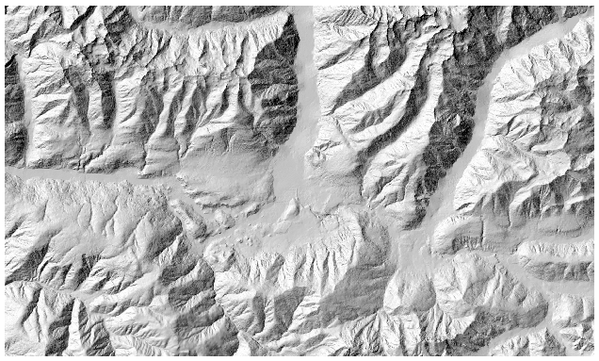
Fig. 23.11 Hillshade layer with azimuth 300 and vertical angle 45
Particularly interesting is to give the hillshade layer a transparency value and overlap it with the elevation raster:
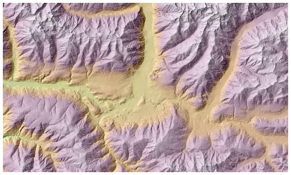
Fig. 23.12 Overlapping the hillshade with the elevation layer
23.1.10.2.1. Parameters
Label |
Name |
Type |
Description |
|---|---|---|---|
Elevation layer |
|
[raster] |
Digital Terrain Model raster layer |
Z factor |
|
[number] Default: 1.0 |
Vertical exaggeration. This parameter is useful when the Z units differ from the X and Y units, for example feet and meters. You can use this parameter to adjust for this. Increasing the value of this parameter will exaggerate the final result (making it look more “hilly”). The default is 1 (no exaggeration). |
Azimuth (horizontal angle) |
|
[number] Default: 300.0 |
Set the horizontal angle (in degrees) of the sun (clockwise direction). Range: 0 to 360. 0 is north. |
Vertical angle |
|
[number] Default: 40.0 |
Set the vertical angle (in degrees) of the sun, that is the height of the sun. Values can go from 0 (minimum elevation) to 90 (maximum elevation). |
Hillshade |
|
[raster] |
Specify the output hillshade raster layer. One of:
The file encoding can also be changed here. |
23.1.10.2.2. Outputs
Label |
Name |
Type |
Description |
|---|---|---|---|
Hillshade |
|
[raster] |
The output hillshade raster layer |
23.1.10.2.3. Python code
Algorithm ID: qgis:hillshade
import processing
processing.run("algorithm_id", {parameter_dictionary})
The algorithm id is displayed when you hover over the algorithm in the Processing Toolbox. The parameter dictionary provides the parameter NAMEs and values. See Using processing algorithms from the console for details on how to run processing algorithms from the Python console.
23.1.10.3. Hypsometric curves
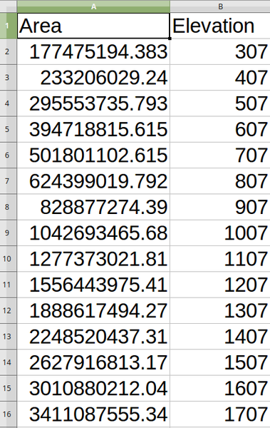
Calculates hypsometric curves for an input Digital Elevation Model. Curves are produced as CSV files in an output folder specified by the user.
A hypsometric curve is a cumulative histogram of elevation values in a geographical area.
You can use hypsometric curves to detect differences in the landscape due to the geomorphology of the territory.
23.1.10.3.1. Parameters
Label |
Name |
Type |
Description |
|---|---|---|---|
DEM to analyze |
|
[raster] |
Digital Terrain Model raster layer to use for calculating altitudes |
Boundary layer |
|
[vector: polygon] |
Polygon vector layer with boundaries of areas used to calculate hypsometric curves |
Step |
|
[number] Default: 100.0 |
Vertical distance between curves |
Use % of area instead of absolute value |
|
[boolean] Default: False |
Write area percentage to “Area” field of the CSV file instead of the absolute area |
Hypsometric curves |
|
[folder] |
Specify the output folder for the hypsometric curves. One of:
The file encoding can also be changed here. |
23.1.10.3.2. Outputs
Label |
Name |
Type |
Description |
|---|---|---|---|
Hypsometric curves |
|
[folder] |
Directory containing the files with the hypsometric curves. For each feature from the input vector layer, a CSV file with area and altitude values will be created. The file names start with |
23.1.10.3.3. Python code
Algorithm ID: qgis:hypsometriccurves
import processing
processing.run("algorithm_id", {parameter_dictionary})
The algorithm id is displayed when you hover over the algorithm in the Processing Toolbox. The parameter dictionary provides the parameter NAMEs and values. See Using processing algorithms from the console for details on how to run processing algorithms from the Python console.
23.1.10.4. Relief
Creates a shaded relief layer from digital elevation data. You can specify the relief color manually, or you can let the algorithm choose automatically all the relief classes.
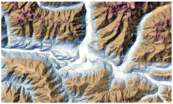
Fig. 23.13 Relief layer
23.1.10.4.1. Parameters
Label |
Name |
Type |
Description |
|---|---|---|---|
Elevation layer |
|
[raster] |
Digital Terrain Model raster layer |
Z factor |
|
[number] Default: 1.0 |
Vertical exaggeration. This parameter is useful when the Z units differ from the X and Y units, for example feet and meters. You can use this parameter to adjust for this. Increasing the value of this parameter will exaggerate the final result (making it look more “hilly”). The default is 1 (no exaggeration). |
Generate relief classes automatically |
|
[boolean] Default: False |
If you check this option the algorithm will create all the relief color classes automatically |
Relief colors Optional |
|
[table widget] |
Use the table widget if you want to choose the relief colors manually. You can add as many color classes as you want: for each class you can choose the lower and upper bound and finally by clicking on the color row you can choose the color thanks to the color widget. 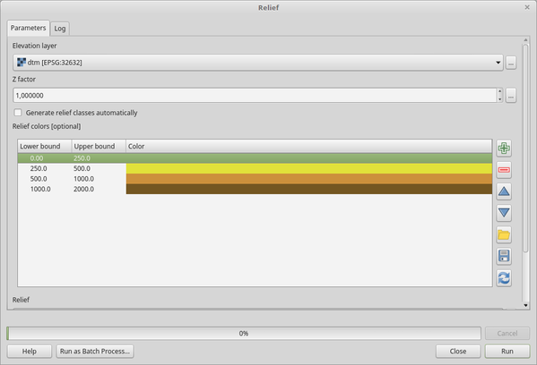
Fig. 23.14 Manually setting of relief color classes The buttons in the right side panel give you the chance to: add or remove color classes, change the order of the color classes already defined, open an existing file with color classes and save the current classes as file. |
Relief |
|
[raster] Default: |
Specify the output relief raster layer. One of:
The file encoding can also be changed here. |
Frequency distribution |
|
[table] Default: |
Specify the CSV table for the output frequency distribution. One of:
The file encoding can also be changed here. |
23.1.10.4.2. Outputs
Label |
Name |
Type |
Description |
|---|---|---|---|
Relief |
|
[raster] |
The output relief raster layer |
Frequency distribution |
|
[table] |
The output frequency distribution |
23.1.10.4.3. Python code
Algorithm ID: qgis:relief
import processing
processing.run("algorithm_id", {parameter_dictionary})
The algorithm id is displayed when you hover over the algorithm in the Processing Toolbox. The parameter dictionary provides the parameter NAMEs and values. See Using processing algorithms from the console for details on how to run processing algorithms from the Python console.
23.1.10.5. Ruggedness index
Calculates the quantitative measurement of terrain heterogeneity described by Riley et al. (1999). It is calculated for every location, by summarizing the change in elevation within the 3x3 pixel grid.
Each pixel contains the difference in elevation from a center cell and the 8 cells surrounding it.
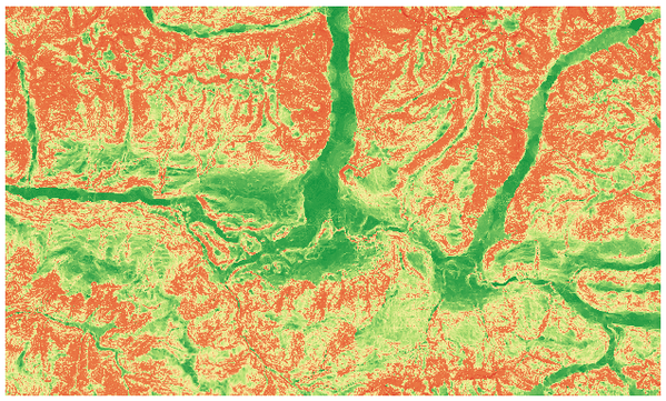
Fig. 23.15 Ruggedness layer from low (red) to high values (green)
23.1.10.5.1. Parameters
Label |
Name |
Type |
Description |
|---|---|---|---|
Elevation layer |
|
[raster] |
Digital Terrain Model raster layer |
Z factor |
|
[number] Default: 1.0 |
Vertical exaggeration. This parameter is useful when the Z units differ from the X and Y units, for example feet and meters. You can use this parameter to adjust for this. Increasing the value of this parameter will exaggerate the final result (making it look more rugged). The default is 1 (no exaggeration). |
Ruggedness |
|
[raster] Default: |
Specify the output ruggedness raster layer. One of:
The file encoding can also be changed here. |
23.1.10.5.2. Outputs
Label |
Name |
Type |
Description |
|---|---|---|---|
Ruggedness |
|
[raster] |
The output ruggedness raster layer |
23.1.10.5.3. Python code
Algorithm ID: qgis:ruggednessindex
import processing
processing.run("algorithm_id", {parameter_dictionary})
The algorithm id is displayed when you hover over the algorithm in the Processing Toolbox. The parameter dictionary provides the parameter NAMEs and values. See Using processing algorithms from the console for details on how to run processing algorithms from the Python console.
23.1.10.6. Slope
Calculates the slope from an input raster layer. The slope is the angle of inclination of the terrain and is expressed in degrees.
In the following picture you can see to the left the DTM layer with the elevation of the terrain while to the right the calculated slope:
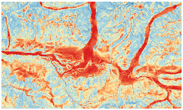
Fig. 23.16 Flat areas in red, steep areas in blue
23.1.10.6.1. Parameters
Label |
Name |
Type |
Description |
|---|---|---|---|
Elevation layer |
|
[raster] |
Digital Terrain Model raster layer |
Z factor |
|
[number] Default: 1.0 |
Vertical exaggeration. This parameter is useful when the Z units differ from the X and Y units, for example feet and meters. You can use this parameter to adjust for this. Increasing the value of this parameter will exaggerate the final result (making it steeper). The default is 1 (no exaggeration). |
Slope |
|
[raster] Default: |
Specify the output slope raster layer. One of:
The file encoding can also be changed here. |
23.1.10.6.2. Outputs
Label |
Name |
Type |
Description |
|---|---|---|---|
Slope |
|
[raster] |
The output slope raster layer |
23.1.10.6.3. Python code
Algorithm ID: qgis:slope
import processing
processing.run("algorithm_id", {parameter_dictionary})
The algorithm id is displayed when you hover over the algorithm in the Processing Toolbox. The parameter dictionary provides the parameter NAMEs and values. See Using processing algorithms from the console for details on how to run processing algorithms from the Python console.