21. Answer Sheet
21.1. Results For Adding Your First Layer
21.1.1.  Preparation
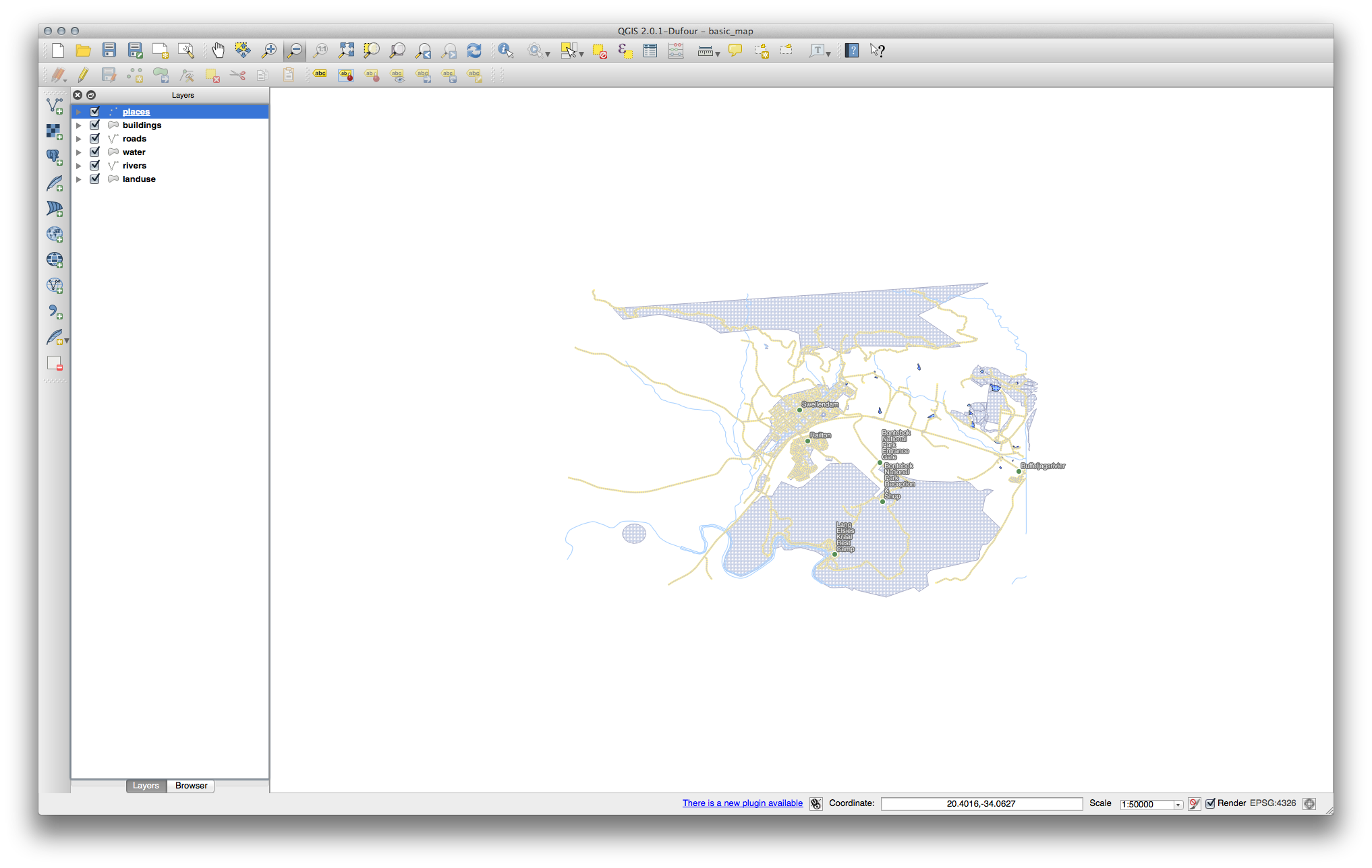
You should see a lot of lines, symbolizing roads. All these lines are in the vector layer that you just loaded to create a basic map.
21.2. Results For An Overview of the Interface
21.2.1. Overview (Part 1)
Refer back to the image showing the interface layout and check that you remember the names and functions of the screen elements.
21.3. Results For Working with Vector Data
21.3.1. Shapefiles
There should be five layers on your map:
- places
- water
- buildings
- rivers and
- roads.
21.3.2. Databases
All the vector layers should be loaded into the map. It probably won’t look nice yet though (we’ll fix the ugly colors later).
21.4. Results For Symbology
21.4.1. Colors
- Verify that the colors are changing as you expect them to change.
- It is enough to change only the water layer for now. An example is below, but may look different depending on the color you chose.
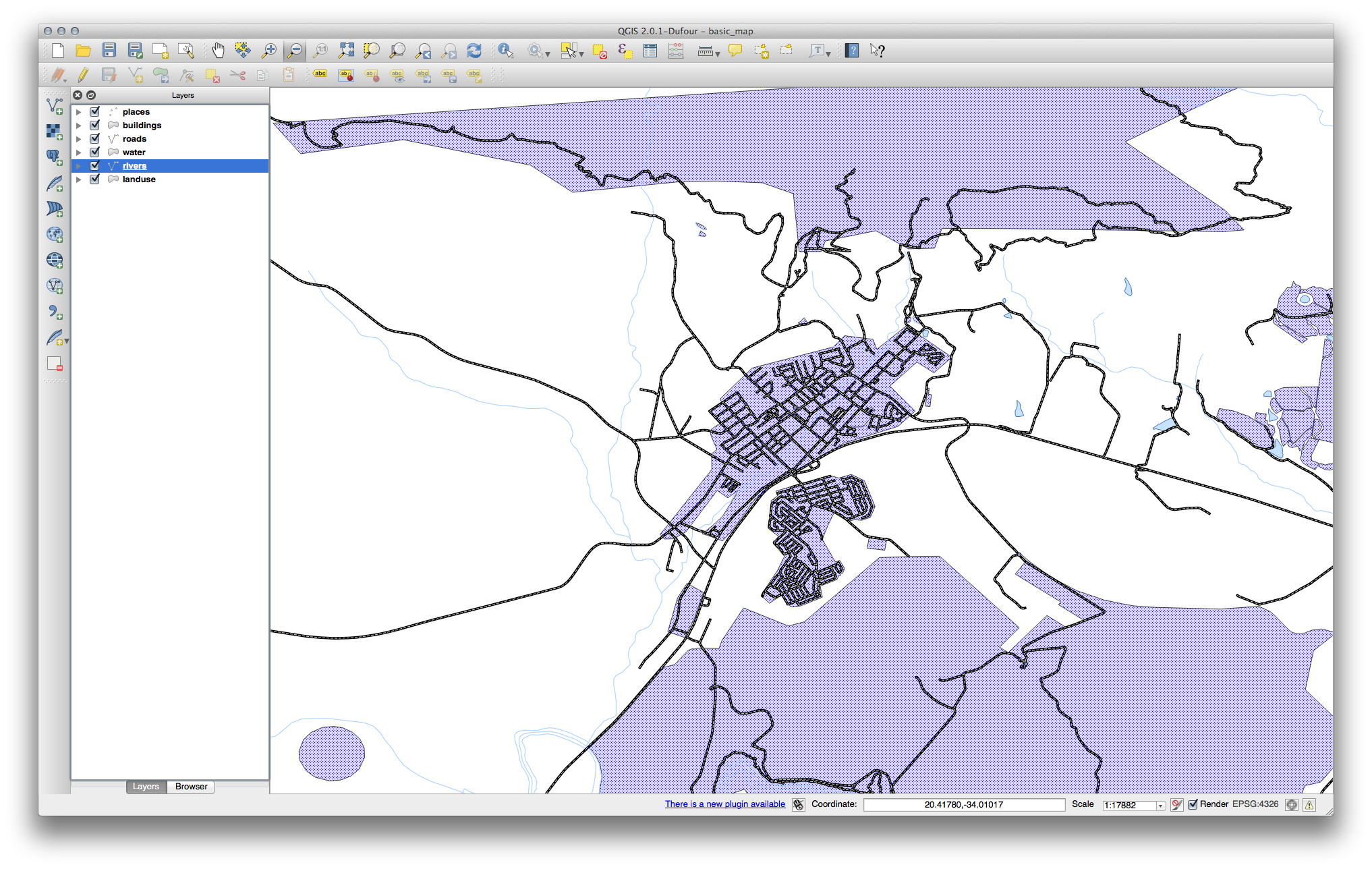
Note
If you want to work on only one layer at a time and don’t want the other layers to distract you, you can hide a layer by clicking in the check box next to its name in the Layers list. If the box is blank, then the layer is hidden.
21.4.2. Symbol Structure
Your map should now look like this:
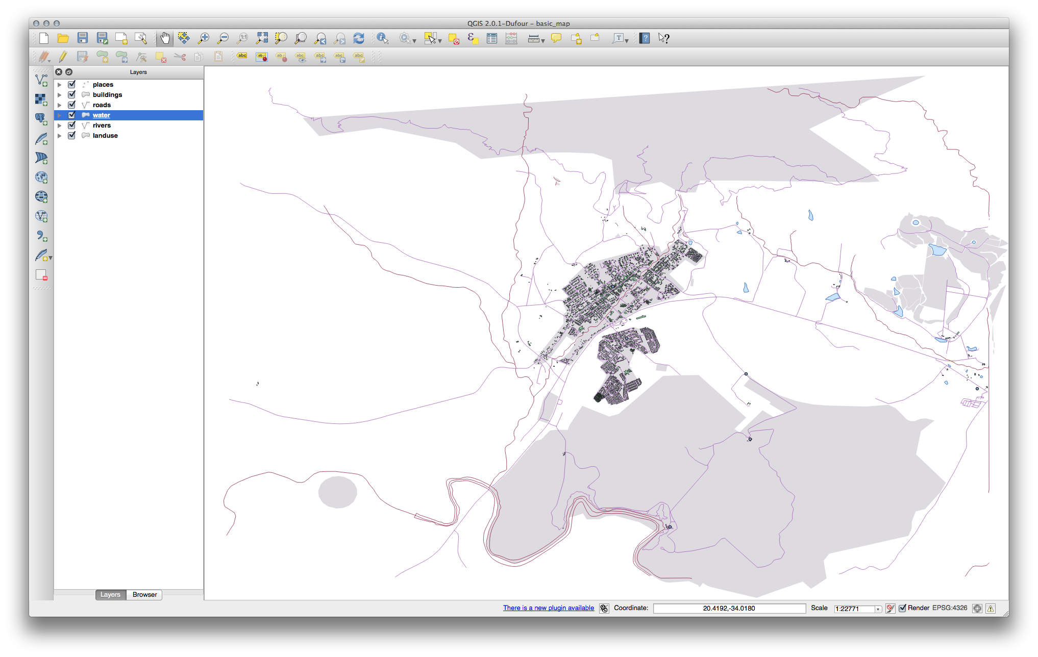
If you are a Beginner-level user, you may stop here.
- Use the method above to change the colors and styles for all the remaining layers.
- Try using natural colors for the objects. For example, a road should not be red or blue, but can be gray or black.
- Also feel free to experiment with different Fill Style and Border Style settings for the polygons.
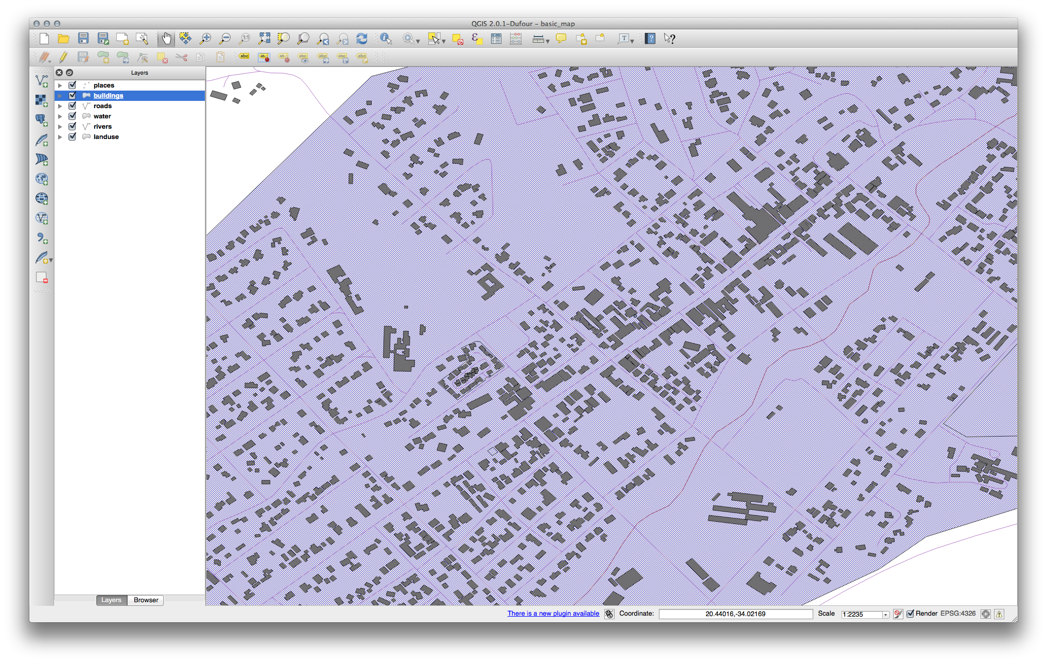
21.4.3.  Symbol Layers
- Customize your buildings layer as you like, but remember that it has to be easy to tell different layers apart on the map.
Here’s an example:
21.4.4. Symbol Levels
To make the required symbol, you need two symbol layers:
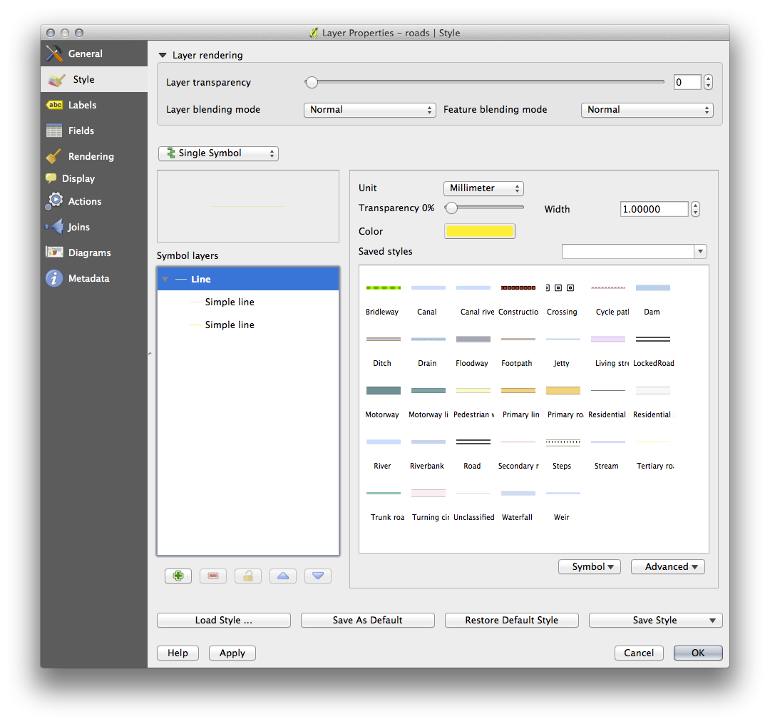
The lowest symbol layer is a broad, solid yellow line. On top of it there is a slightly thinner solid gray line.
If your symbol layers resemble the above but you’re not getting the result you want, check that your symbol levels look something like this:
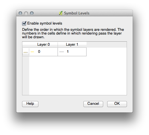
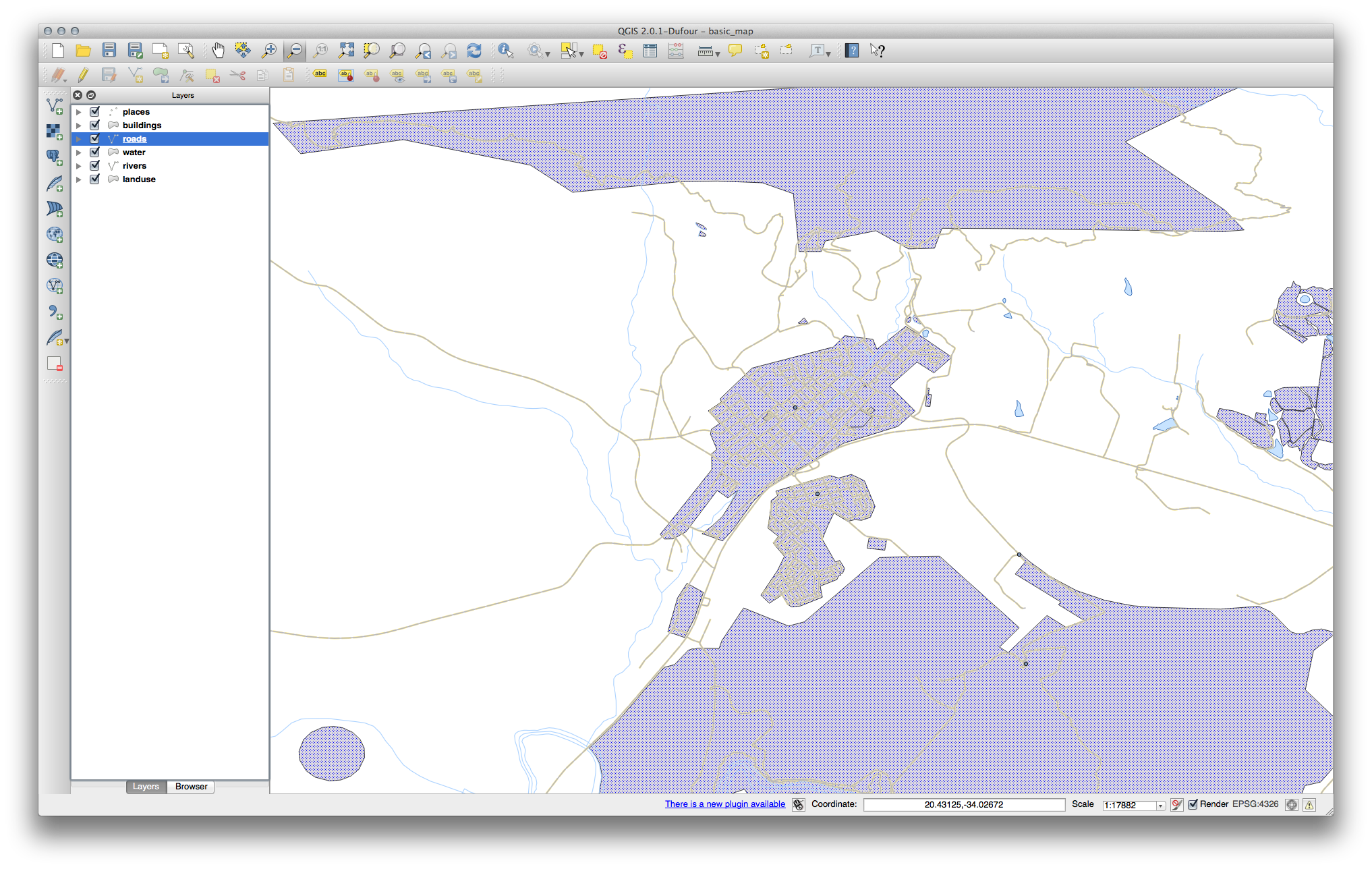
Now your map should look like this:
21.4.5.  Symbol Levels
- Adjust your symbol levels to these values:
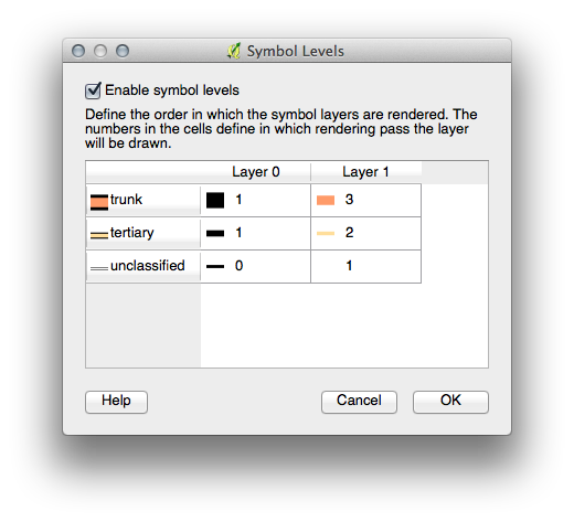
- Experiment with different values to get different results.
- Open your original map again before continuing with the next exercise.
21.5. Results For Attribute Data
21.5.1. Attribute Data
The NAME field is the most useful to show as labels. This is because all its values are unique for every object and are very unlikely to contain NULL values. If your data contains some NULL values, do not worry as long as most of your places have names.
21.6. Results For The Label Tool
21.6.1. Label Customization (Part 1)
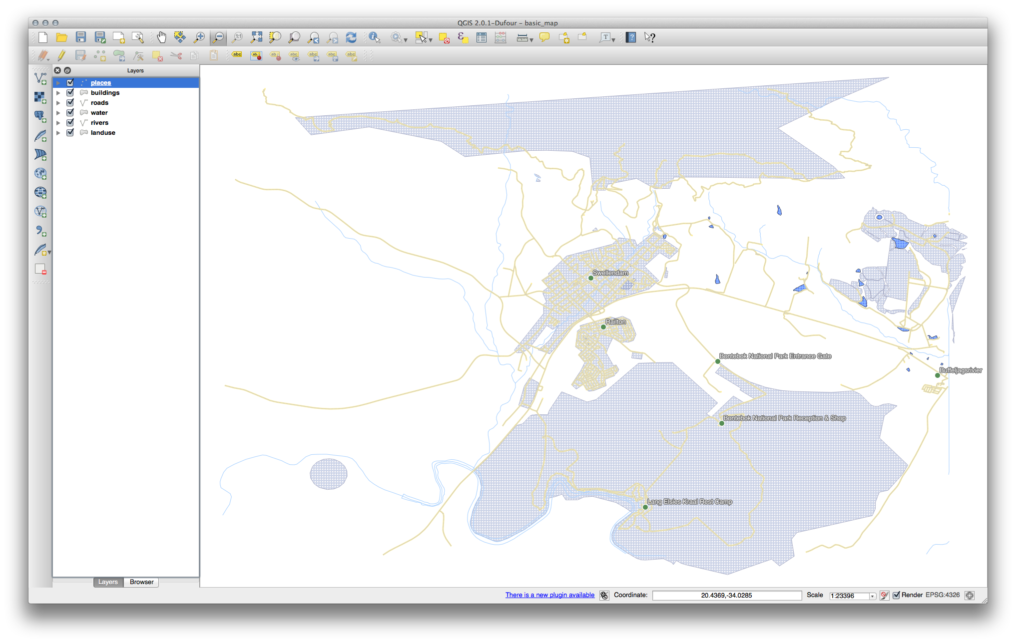
Your map should now show the marker points and the labels should be offset by 2.0 mm: The style of the markers and labels should allow both to be clearly visible on the map:
21.6.2. Label Customization (Part 2)
One possible solution has this final product:
To arrive at this result:
Use a font size of 10, a Label distance of 1,5 mm, Symbol width and Symbol size of 3.0 mm.
In addition, this example uses the Wrap label on character option:
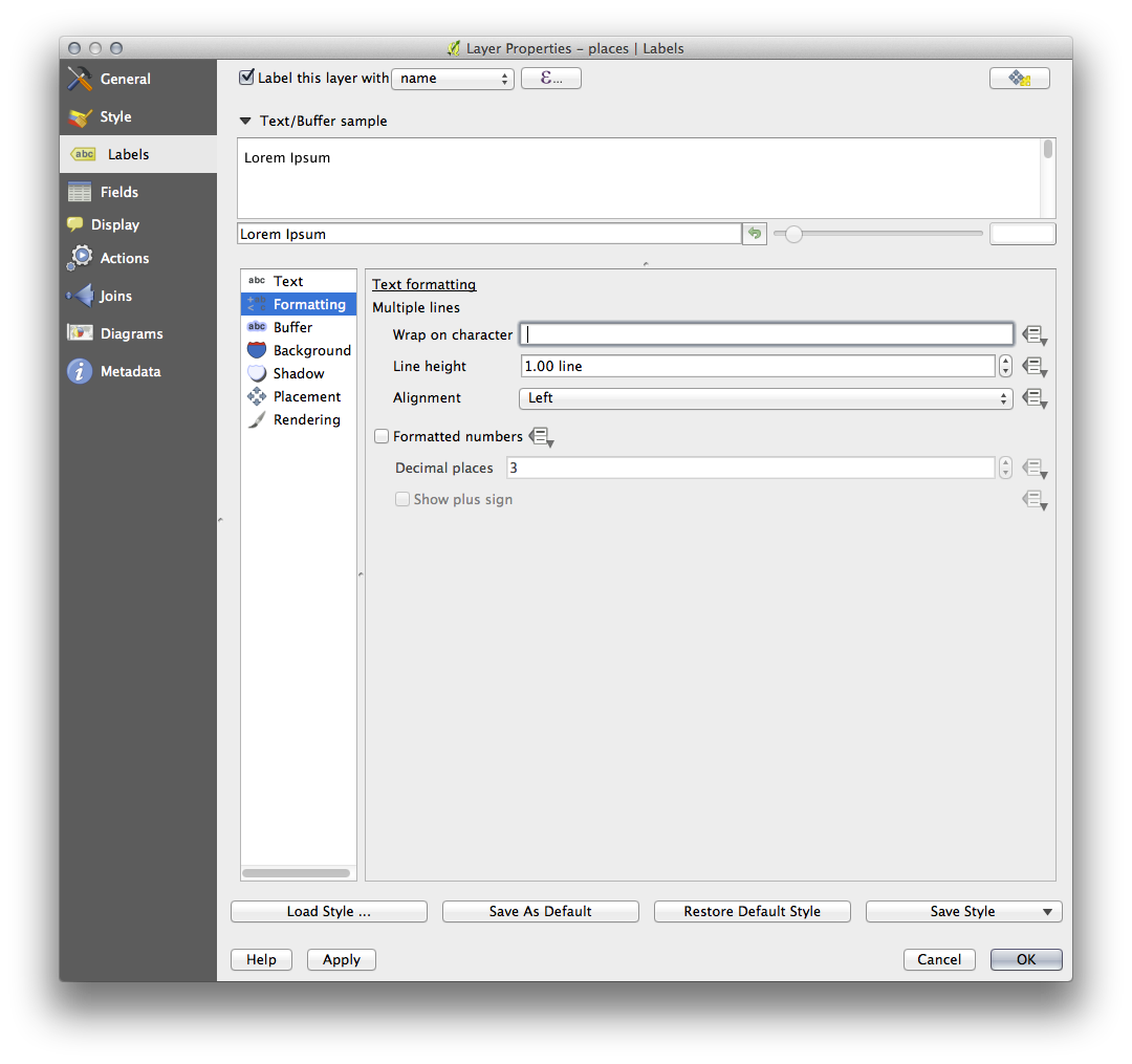
Enter a space in this field and click Apply to achieve the same effect. In our case, some of the place names are very long, resulting in names with multiple lines which is not very user friendly. You might find this setting to be more appropriate for your map.
21.6.3. Using Data Defined Settings
Still in edit mode, set the FONT_SIZE values to whatever you prefer. The example uses 16 for towns, 14 for suburbs, 12 for localities and 10 for hamlets.
Remember to save changes and exit edit mode.
Return to the Text formatting options for the places layer and select FONT_SIZE in the Attribute field of the font size data override dropdown:
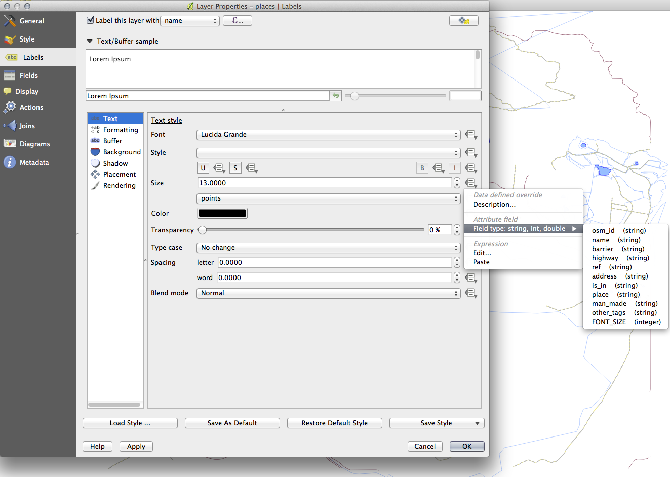
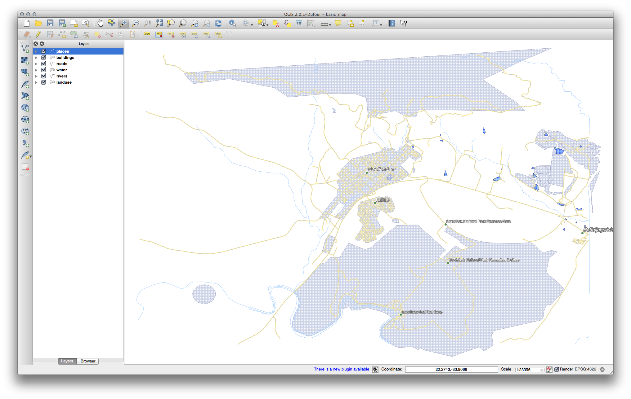
Your results, if using the above values, should be this:
21.7. Results For Classification
21.7.1. Refine the Classification
Use the same method as in the first exercise of the lesson to get rid of the borders:
The settings you used might not be the same, but with the values Classes = 6 and Mode = Natural Breaks (Jenks) (and using the same colors, of course), the map will look like this:
21.8. Results For Creating a New Vector Dataset
21.8.1. Digitizing
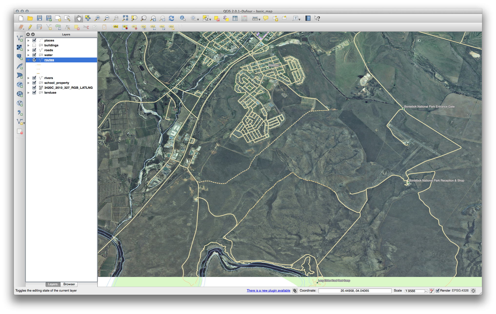
The symbology doesn’t matter, but the results should look more or less like this:
21.8.2. Topology: Add Ring Tool
The exact shape doesn’t matter, but you should be getting a hole in the middle of your feature, like this one:
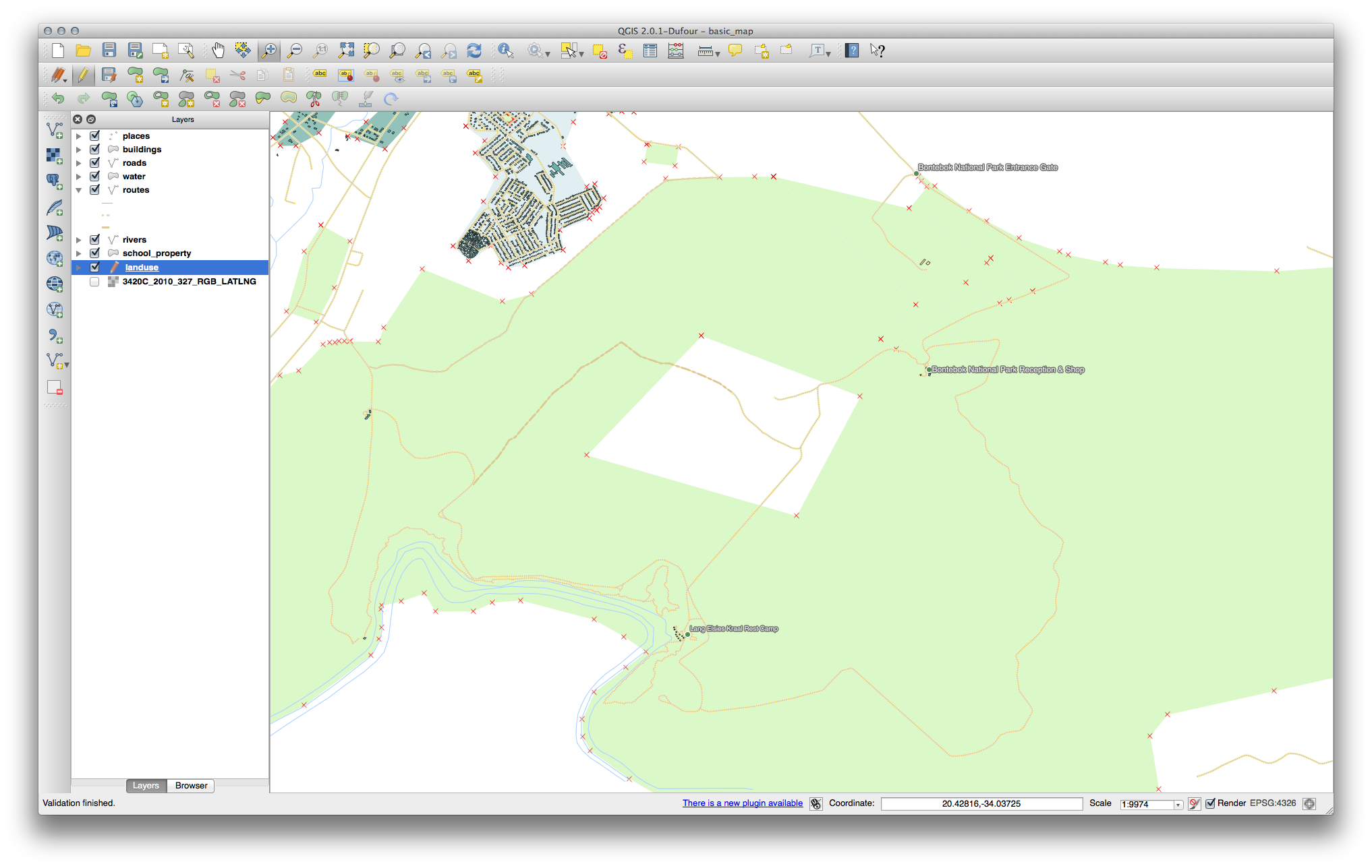
- Undo your edit before continuing with the exercise for the next tool.
21.8.3. Topology: Add Part Tool
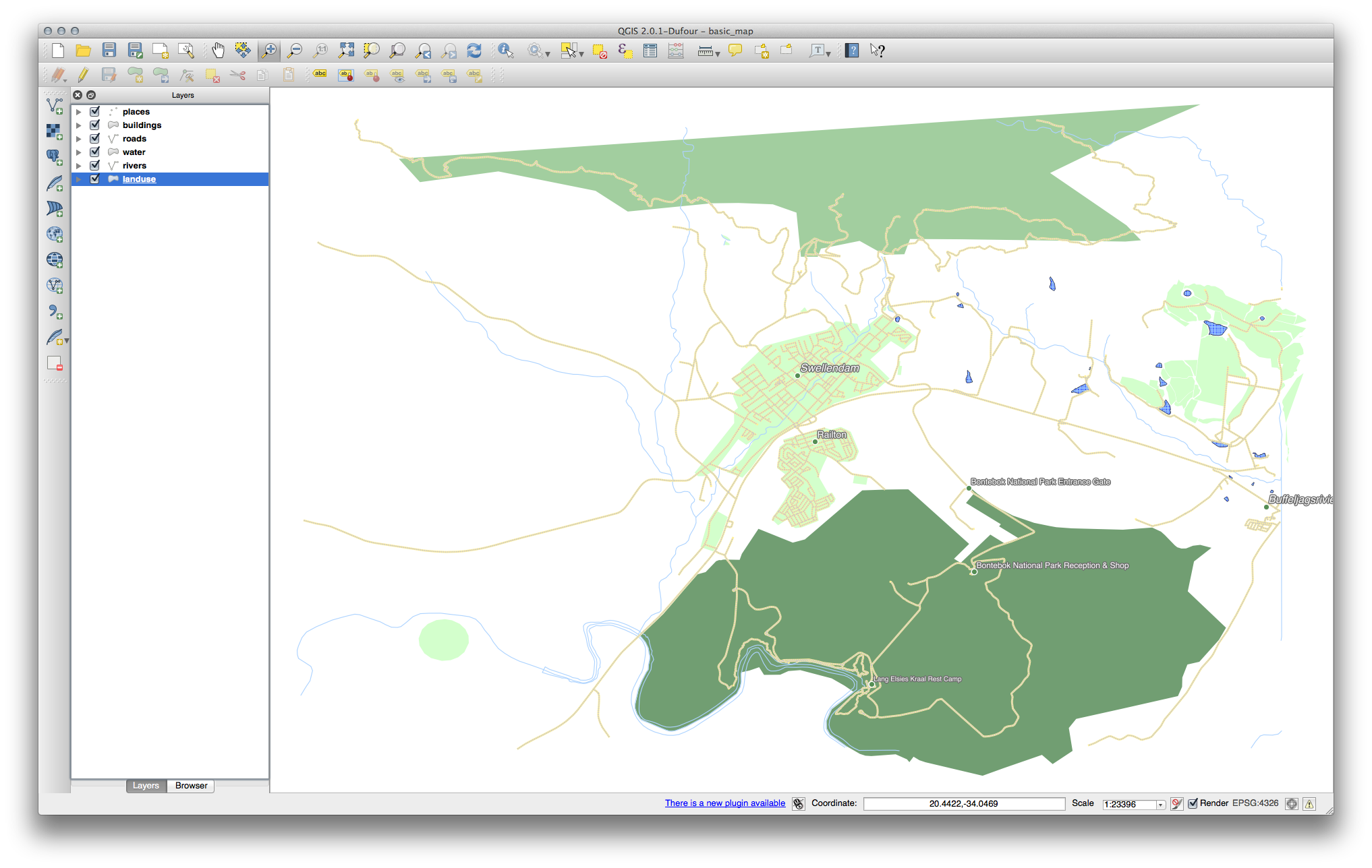
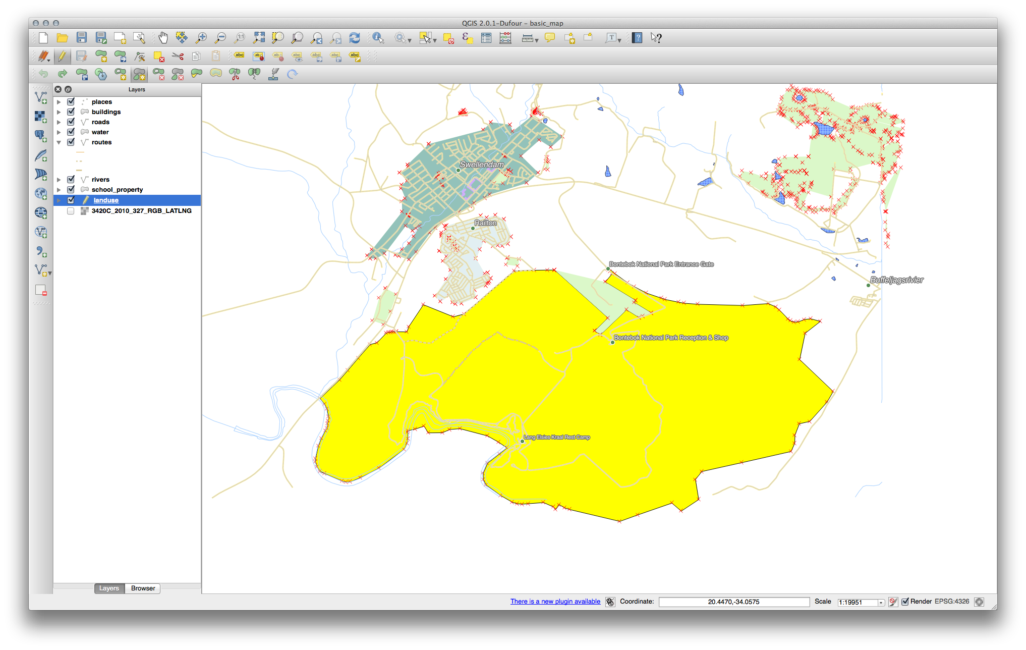
- First select the Bontebok National Park:
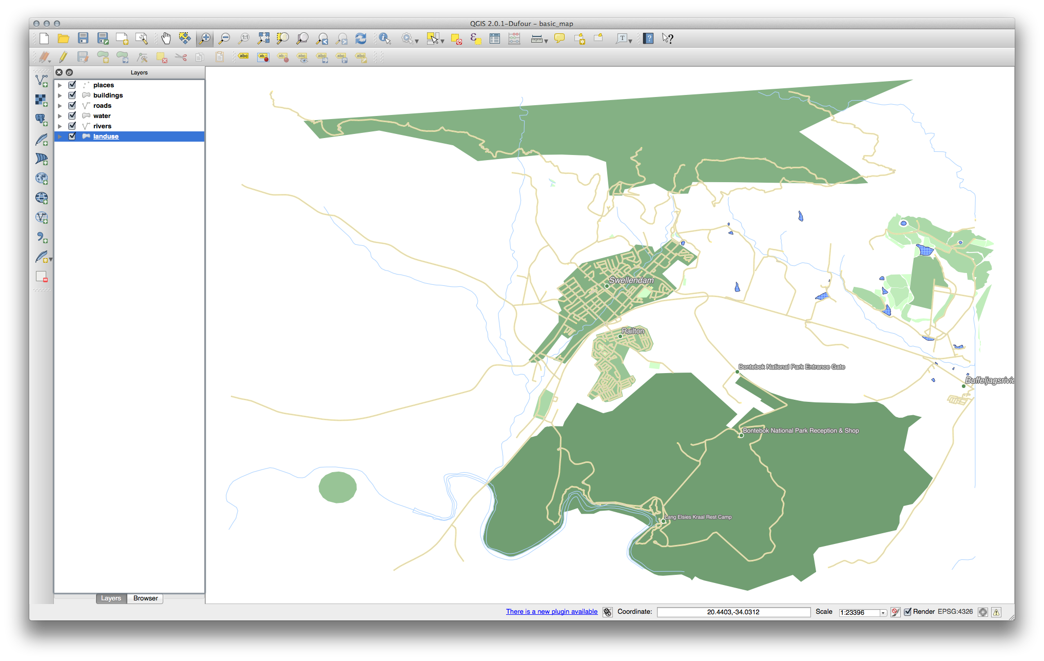
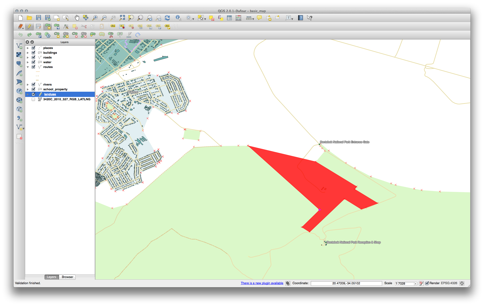
- Now add your new part:
- Undo your edit before continuing with the exercise for the next tool.
21.8.4. Merge Features
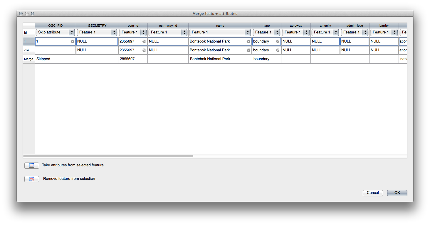
- Use the Merge Selected Features tool, making sure to first select both of the polygons you wish to merge.
- Use the feature with the OGC_FID of 1 as the source of your attributes (click on its entry in the dialog, then click the Take attributes from selected feature button):
Note
- If you’re using a different dataset, it is highly likely that your
- original polygon’s OGC_FID will not be 1. Just choose the feature which has an OGC_FID.
Note
Using the Merge Attributes of Selected Features tool will keep the geometries distinct, but give them the same attributes.
21.8.5. Forms
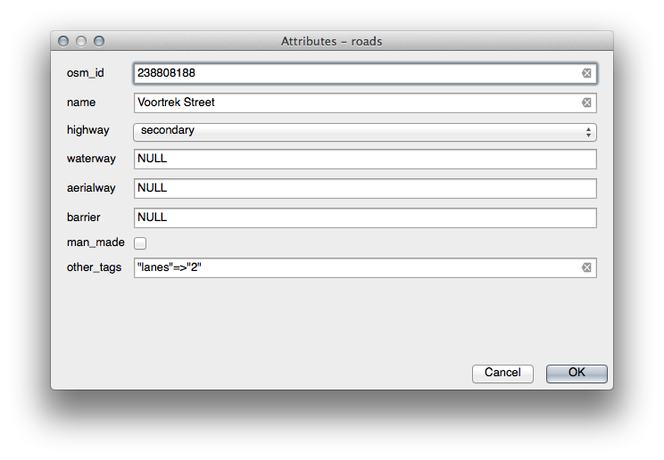
For the TYPE, there is obviously a limited amount of types that a road can be, and if you check the attribute table for this layer, you’ll see that they are predefined.
Set the widget to Value Map and click Load Data from Layer.
Select roads in the Label dropdown and highway for both the Value and Description options:
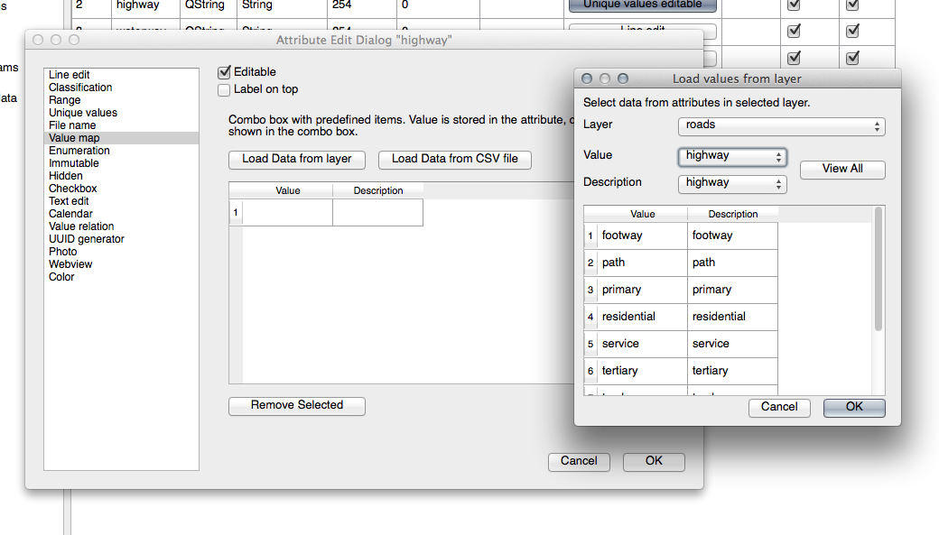
Click Ok three times.
If you use the Identify tool on a street now while edit mode is active, the dialog you get should look like this:
21.9. Results For Vector Analysis
21.9.1. Extract Your Layers from OSM Data
For the purpose of this exercise, the OSM layers which we are interested in are multipolygons and lines. The multipolygons layer contains the data we need in order to produce the houses, schools and restaurants layers. The lines layer contains the roads dataset.
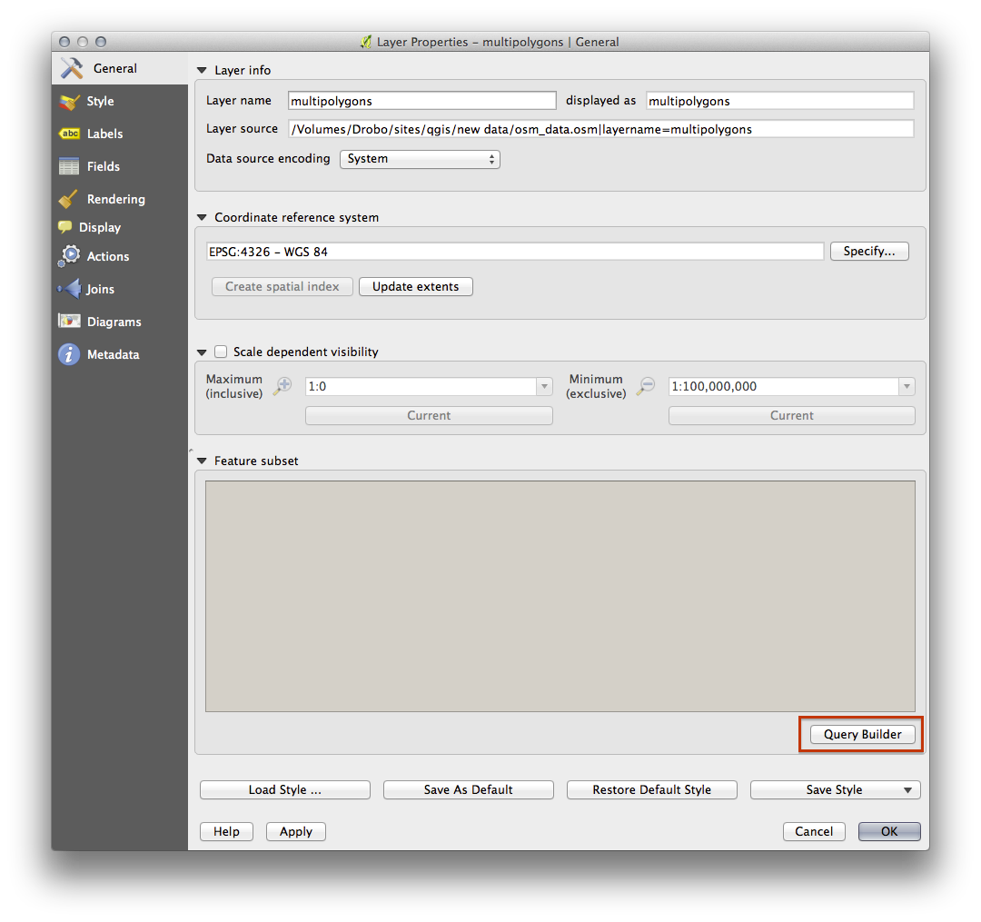
The Query Builder is found in the layer properties:
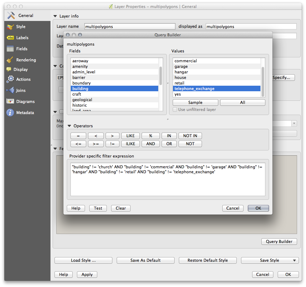
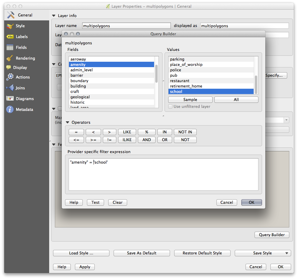
Using the Query Builder against the multipolygons layer, create the following queries for the houses, schools, restaurants and residential layers:
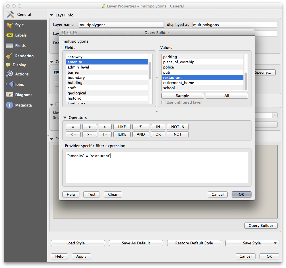
Once you have entered each query, click OK. You’ll see that the map updates to show only the data you have selected. Since you need to use again the multipolygons data from the OSM dataset, at this point, you can use one of the following methods:
- Rename the filtered OSM layer and re-import the layer from osm_data.osm, OR
- Duplicate the filtered layer, rename the copy, clear the query and create your new query in the Query Builder.
Note
Although OSM’s building field has a house value, the coverage in your area - as in ours - may not be complete. In our test region, it is therefore more accurate to exclude all buildings which are defined as anything other than house. You may decide to simply include buildings which are defined as house and all other values that have not a clear meaning like yes.
To create the roads layer, build this query against OSM’s lines layer:
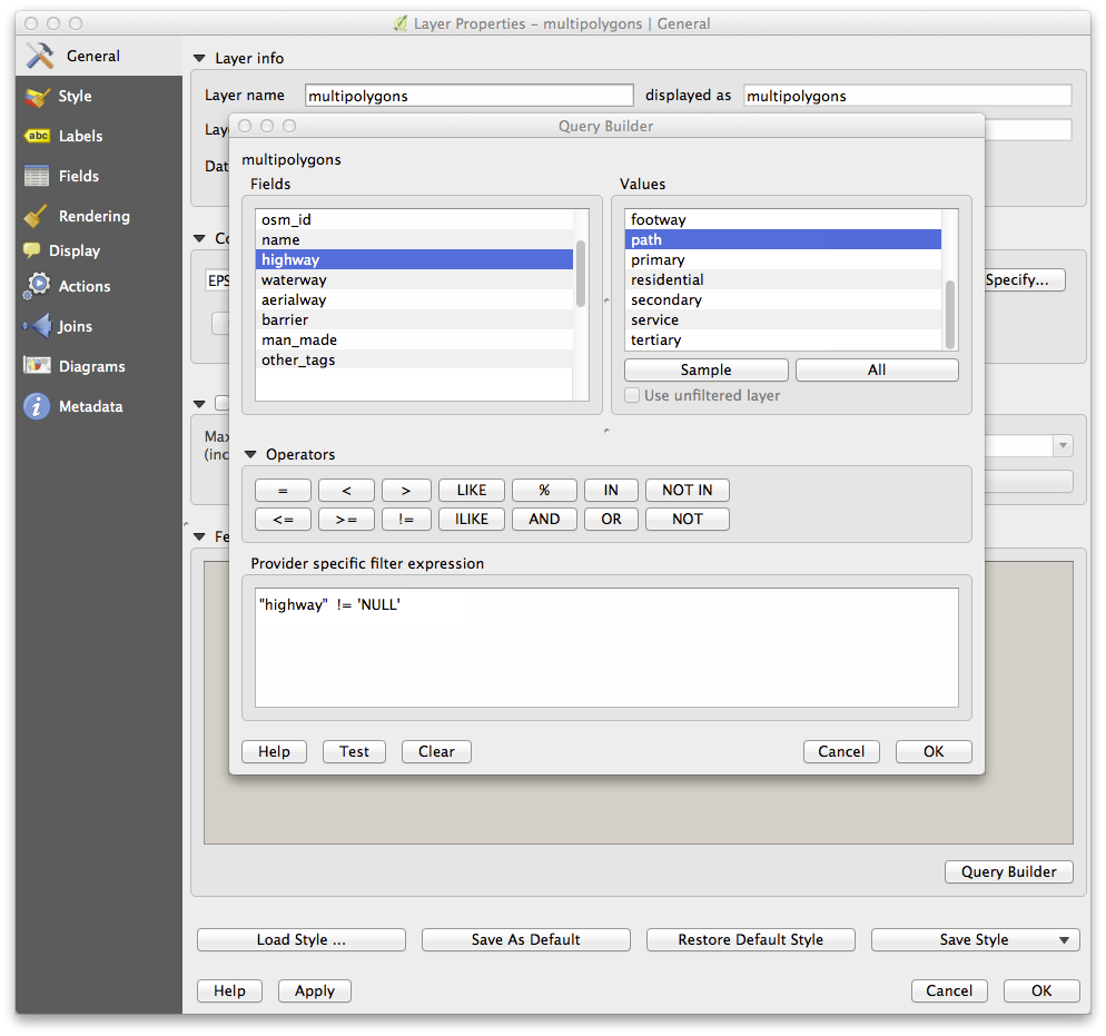
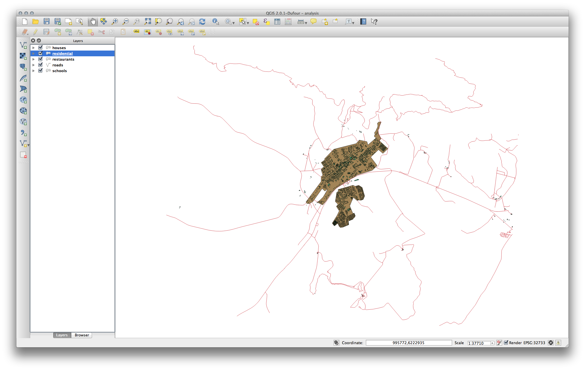
You should end up with a map which looks similar to the following:
21.9.2. Distance from High Schools
Your buffer dialog should look like this:
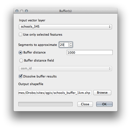
The Buffer distance is 1000 meters (i.e., 1 kilometer).
The Segments to approximate value is set to 20. This is optional, but it’s recommended, because it makes the output buffers look smoother. Compare this:
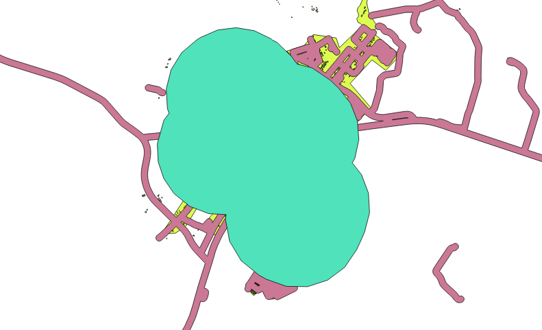
To this:
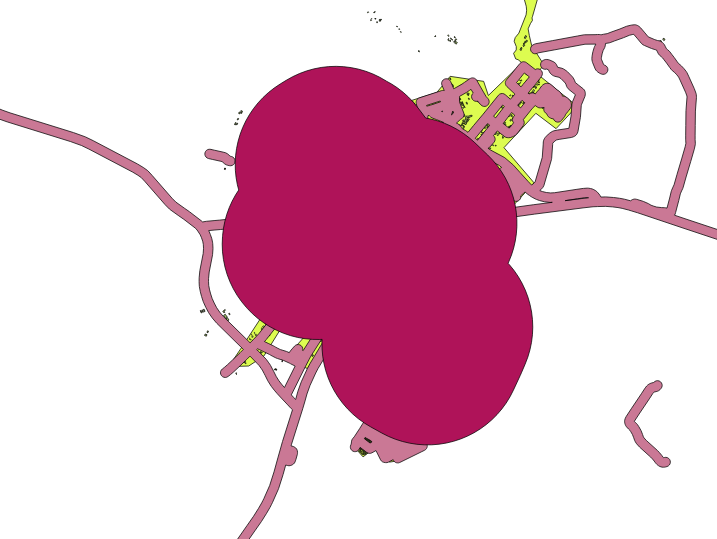
The first image shows the buffer with the Segments to approximate value set to 5 and the second shows the value set to 20. In our example, the difference is subtle, but you can see that the buffer’s edges are smoother with the higher value.
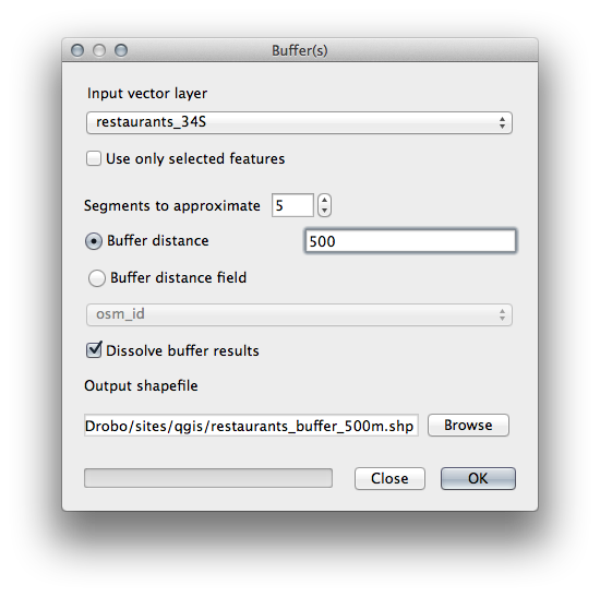
21.9.3. Distance from Restaurants
To create the new houses_restaurants_500m layer, we go through a two step process:
First, create a buffer of 500m around the restaurants and add the layer to the map:
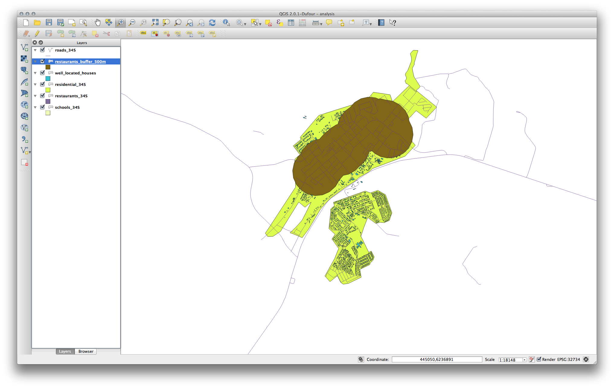
Next, select buildings within that buffer area:
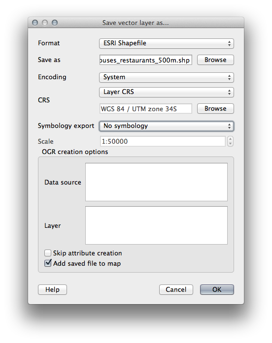
Now save that selection to our new houses_restaurants_500m layer:
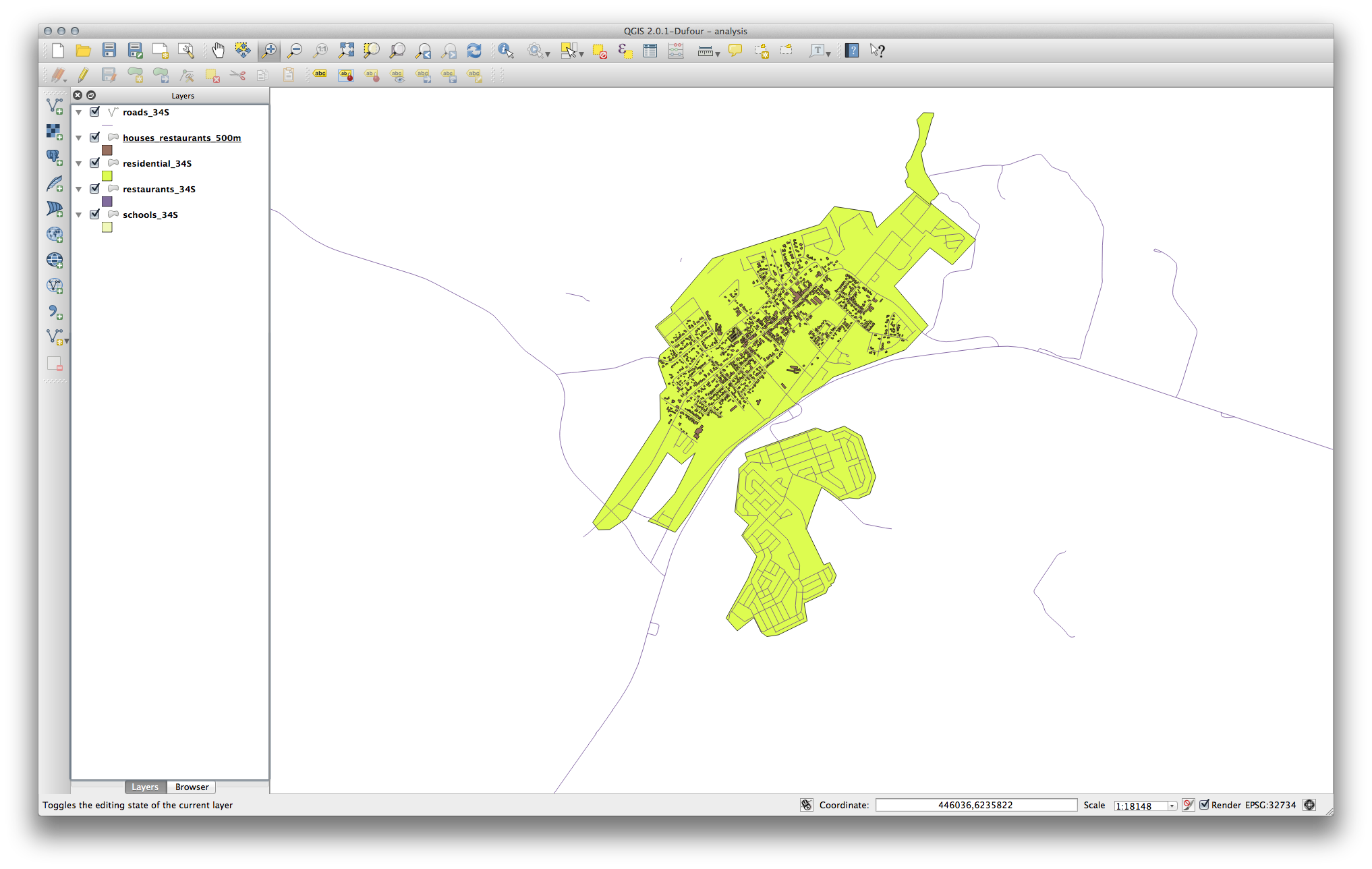
Your map should now show only those buildings which are within 50m of a road, 1km of a school and 500m of a restaurant:
21.10. Results For Raster Analysis
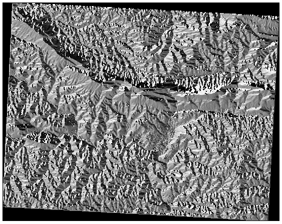
21.10.2. Calculate Slope (less than 2 and 5 degrees)
Set your Raster calculator dialog up like this:
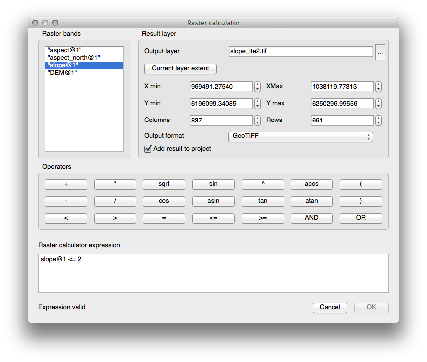
For the 5 degree version, replace the 2 in the expression and file name with 5.
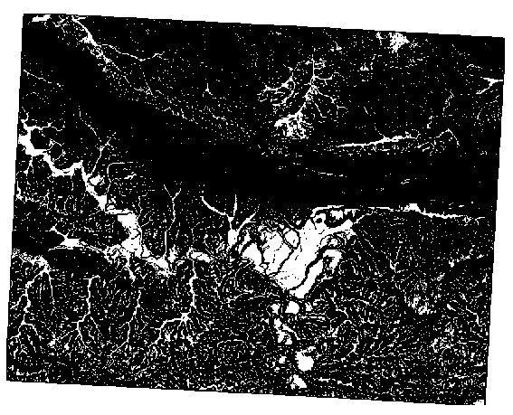
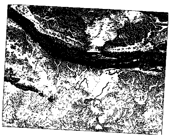
Your results:
2 degrees:
5 degrees:
21.11. Results For Completing the Analysis
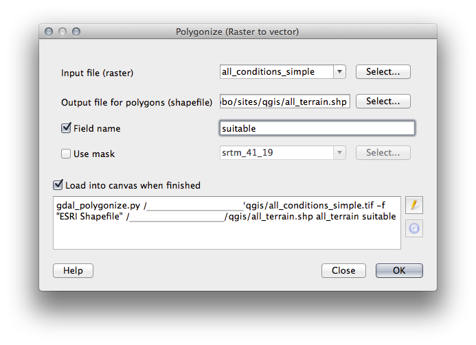
21.11.1. Raster to Vector
- Open the Query Builder by right-clicking on the all_terrain layer in the Layers list, select the General tab.
- Then build the query "suitable" = 1.
- Click OK to filter out all the polygons where this condition isn’t met.
When viewed over the original raster, the areas should overlap perfectly:
- You can save this layer by right-clicking on the all_terrain layer in the Layers list and choosing Save As..., then continue as per the instructions.
21.11.2. Inspecting the Results
You may notice that some of the buildings in your new_solution layer have been “sliced” by the Intersect tool. This shows that only part of the building - and therefore only part of the property - lies on suitable terrain. We can therefore sensibly eliminate those buildings from our dataset
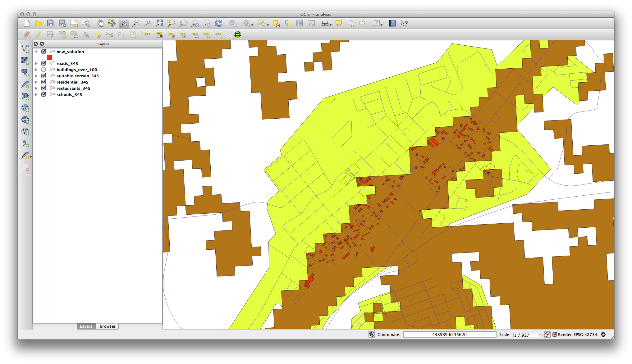
21.11.3. Refining the Analysis
At the moment, your analysis should look something like this:
Consider a circular area, continuous for 100 meters in all directions.
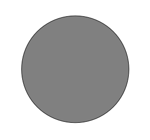
If it is greater than 100 meters in radius, then subtracting 100 meters from its size (from all directions) will result in a part of it being left in the middle.
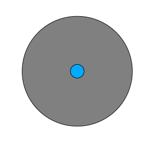
Therefore, you can run an interior buffer of 100 meters on your existing suitable_terrain vector layer. In the output of the buffer function, whatever remains of the original layer will represent areas where there is suitable terrain for 100 meters beyond.
To demonstrate:
Go to Vector ‣ Geoprocessing Tools ‣ Buffer(s) to open the Buffer(s) dialog.
Set it up like this:
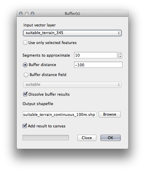
Use the suitable_terrain layer with 10 segments and a buffer distance of -100. (The distance is automatically in meters because your map is using a projected CRS.)
Save the output in exercise_data/residential_development/ as suitable_terrain_continuous100m.shp.
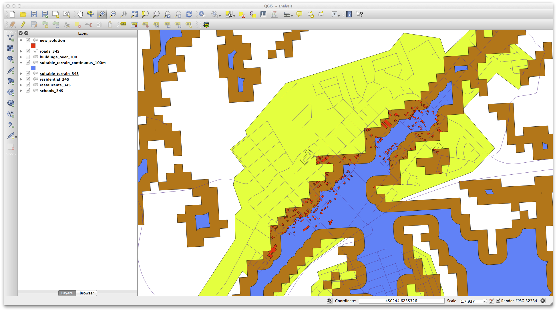
If necessary, move the new layer above your original suitable_terrain layer.
Your results will look like something like this:
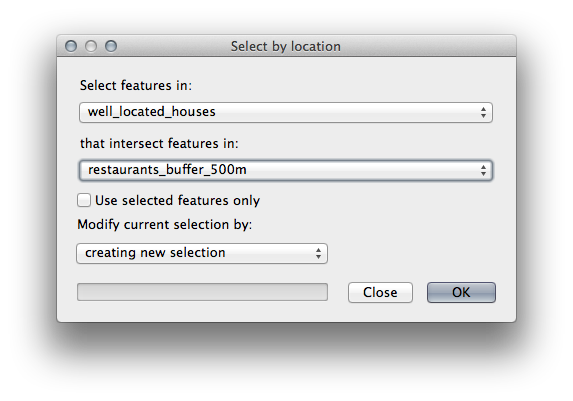
Now use the Select by Location tool (Vector ‣ Research Tools ‣ Select by location).
Set up like this:
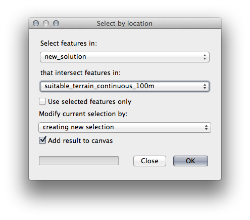
Select features in new_solution that intersect features in suitable_terrain_continuous100m.shp.
This is the result:

The yellow buildings are selected. Although some of the buildings fall partly outside the new suitable_terrain_continuous100m layer, they lie well within the original suitable_terrain layer and therefore meet all of our requirements.
- Save the selection under exercise_data/residential_development/ as final_answer.shp.
21.12. Results For WMS
21.12.1. Adding Another WMS Layer
Your map should look like this (you may need to re-order the layers):
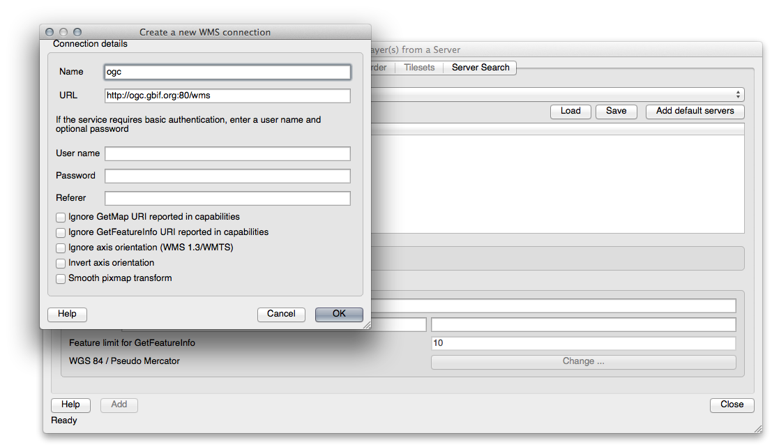
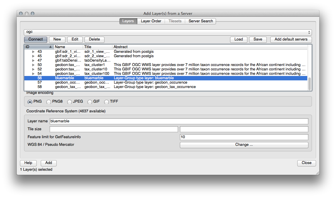
21.12.2. Adding a New WMS Server
Use the same approach as before to add the new server and the appropriate layer as hosted on that server:
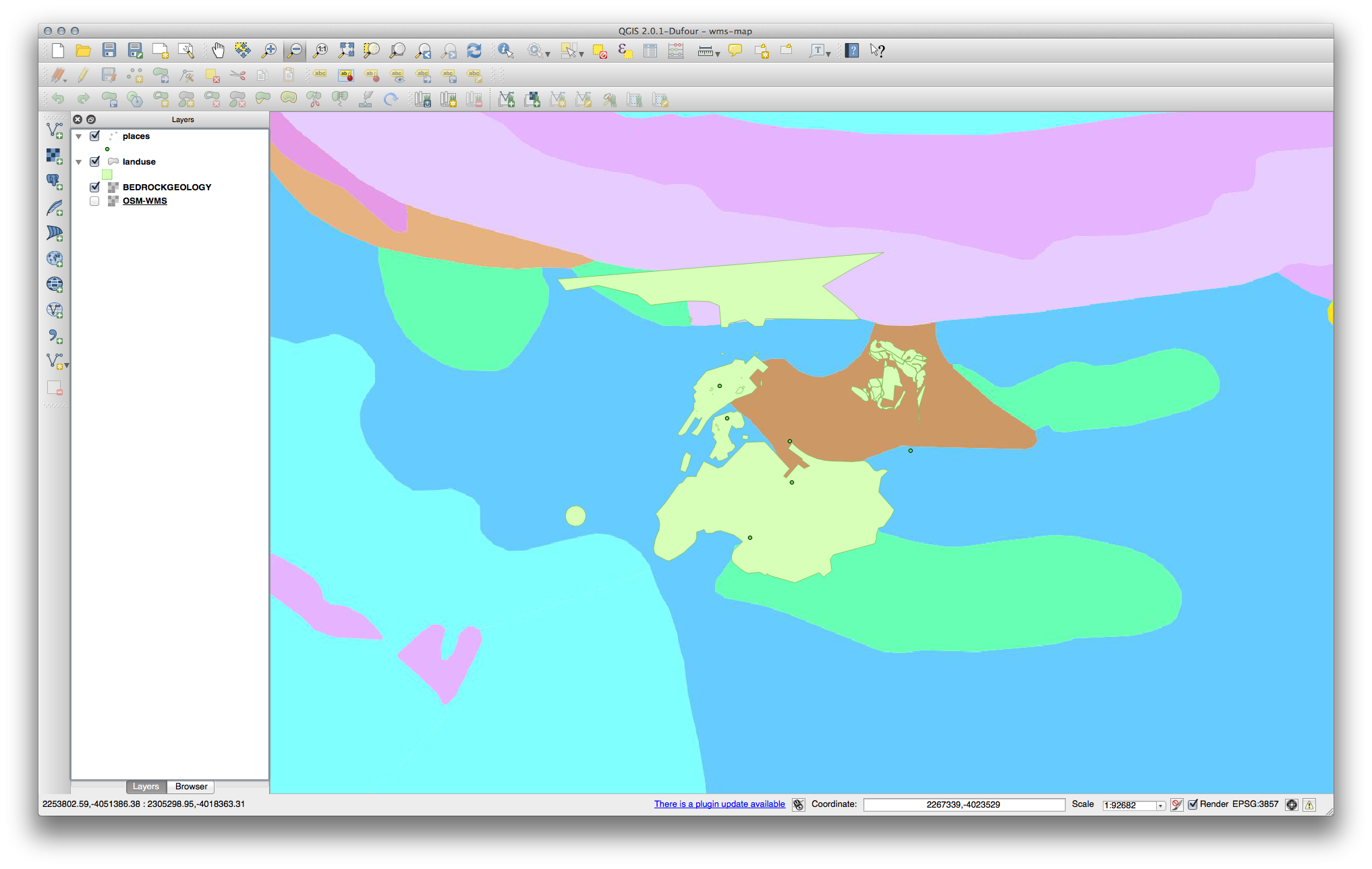
If you zoom into the Swellendam area, you’ll notice that this dataset has a low resolution:
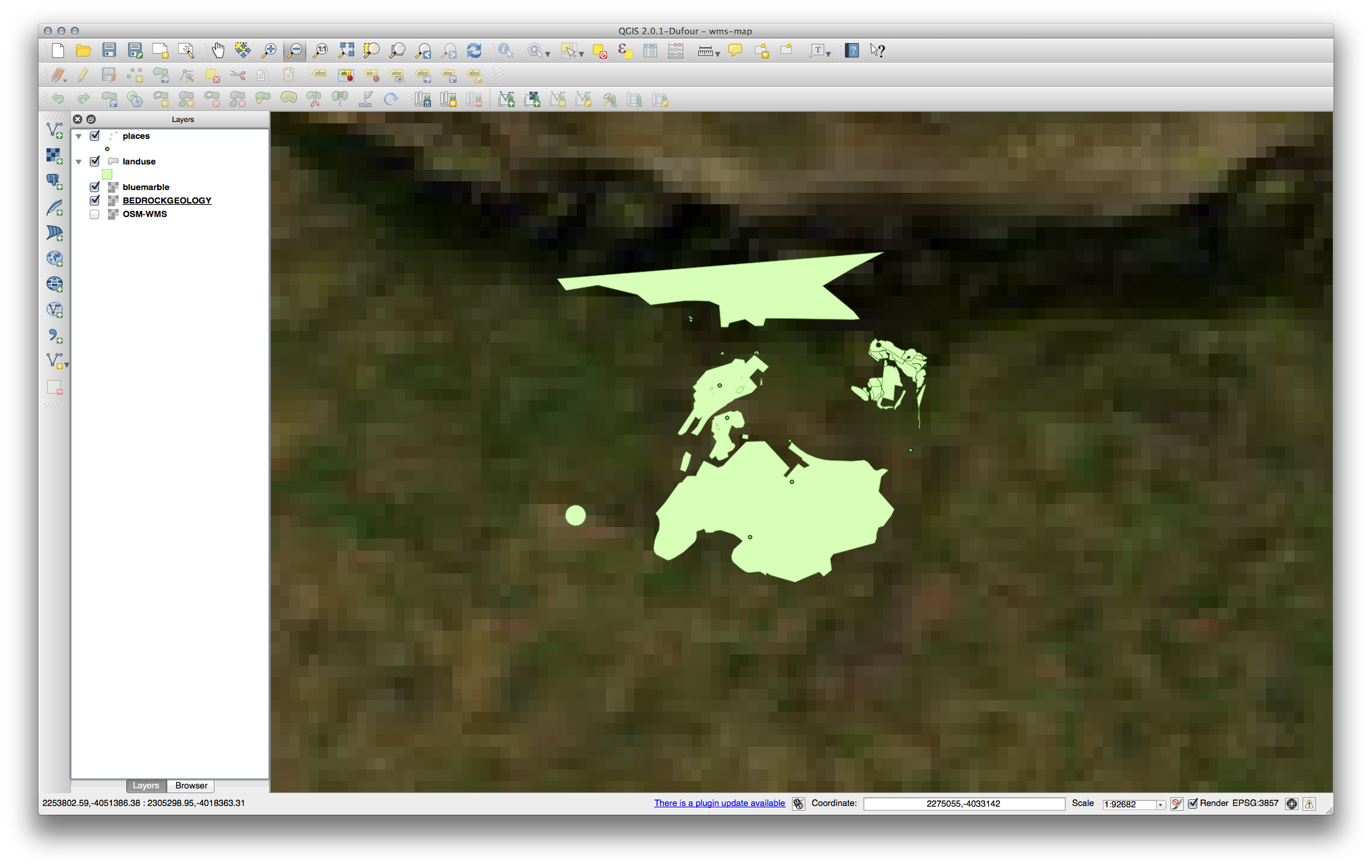
Therefore, it’s better not to use this data for the current map. The Blue Marble data is more suitable at global or national scales.
21.12.3. Finding a WMS Server
You may notice that many WMS servers are not always available. Sometimes this is temporary, sometimes it is permanent. An example of a WMS server that worked at the time of writing is the World Mineral Deposits WMS at http://apps1.gdr.nrcan.gc.ca/cgi-bin/worldmin_en-ca_ows. It does not require fees or have access constraints, and it is global. Therefore, it does satisfy the requirements. Keep in mind, however, that this is merely an example. There are many other WMS servers to choose from.
21.13. Results For Database Concepts
21.13.1. Address Table Properties
For our theoretical address table, we might want to store the following properties:
House Number
Street Name
Suburb Name
City Name
Postcode
Country
When creating the table to represent an address object, we would create columns to represent each of these properties and we would name them with SQL-compliant and possibly shortened names:
house_number
street_name
suburb
city
postcode
country
21.13.2. Normalising the People Table
The major problem with the people table is that there is a single address field which contains a person’s entire address. Thinking about our theoretical address table earlier in this lesson, we know that an address is made up of many different properties. By storing all these properties in one field, we make it much harder to update and query our data. We therefore need to split the address field into the various properties. This would give us a table which has the following structure:
id |     name      | house_no |  street_name   |    city    |   phone_no
 --+---------------+----------+----------------+------------+-----------------
 1 | Tim Sutton    |     3    | Buirski Plein  | Swellendam | 071 123 123
 2 | Horst Duester |     4    | Avenue du Roix | Geneva     | 072 121 122
Note
In the next section, you will learn about Foreign Key relationships which could be used in this example to further improve our database’s structure.
21.13.3. Further Normalisation of the People Table
Our people table currently looks like this:
id |     name     | house_no | street_id |  phone_no
---+--------------+----------+-----------+-------------
 1 | Horst Duster |        4 |         1 | 072 121 122
The street_id column represents a ‘one to many’ relationship between the people object and the related street object, which is in the streets table.
One way to further normalise the table is to split the name field into first_name and last_name:
id | first_name | last_name  | house_no | street_id |  phone_no
---+------------+------------+----------+-----------+------------
 1 |    Horst   |   Duster   |     4    |     1     | 072 121 122
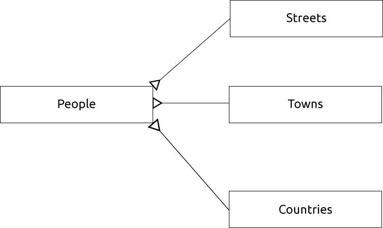
We can also create separate tables for the town or city name and country, linking them to our people table via ‘one to many’ relationships:
id | first_name | last_name | house_no | street_id | town_id | country_id
---+------------+-----------+----------+-----------+---------+------------
 1 |    Horst   |   Duster  |     4    |     1     |    2    |     1
An ER Diagram to represent this would look like this:
21.13.4. Create a People Table
The SQL required to create the correct people table is:
create table people (id serial not null primary key,
                     name varchar(50),
                     house_no int not null,
                     street_id int not null,
                     phone_no varchar null );
The schema for the table (enter \d people) looks like this:
Table "public.people"

Column     |         Type          |                      Modifiers
-----------+-----------------------+-------------------------------------
id         | integer               | not null default
           |                       | nextval('people_id_seq'::regclass)
name       | character varying(50) |
house_no   | integer               | not null
street_id  | integer               | not null
phone_no   | character varying     |
Indexes:
  "people_pkey" PRIMARY KEY, btree (id)
Note
For illustration purposes, we have purposely omitted the fkey constraint.
21.13.5. The DROP Command
The reason the DROP command would not work in this case is because the people table has a Foreign Key constraint to the streets table. This means that dropping (or deleting) the streets table would leave the people table with references to non-existent streets data.
Note
It is possible to ‘force’ the streets table to be deleted by using the CASCADE command, but this would also delete the people and any other table which had a relationship to the streets table. Use with caution!
21.13.6. Insert a New Street
The SQL command you should use looks like this (you can replace the street name with a name of your choice):
insert into streets (name) values ('Low Road');
21.13.7. Add a New Person With Foreign Key Relationship
Here is the correct SQL statement:
insert into streets (name) values('Main Road');
insert into people (name,house_no, street_id, phone_no)
  values ('Joe Smith',55,2,'072 882 33 21');
If you look at the streets table again (using a select statement as before), you’ll see that the id for the Main Road entry is 2.
That’s why we could merely enter the number 2 above. Even though we’re not seeing Main Road written out fully in the entry above, the database will be able to associate that with the street_id value of 2.
Note
If you have already added a new street object, you might find that the new Main Road has an ID of 3 not 2.
21.13.8. Return Street Names
Here is the correct SQL statement you should use:
select count(people.name), streets.name
from people, streets
where people.street_id=streets.id
group by streets.name;
Result:
count |    name
------+-------------
    1 | Low Street
    2 | High street
    1 | Main Road
(3 rows)
Note
You will notice that we have prefixed field names with table names (e.g. people.name and streets.name). This needs to be done whenever the field name is ambiguous (i.e. not unique across all tables in the database).
21.14. Results For Spatial Queries
21.14.1. The Units Used in Spatial Queries
The units being used by the example query are degrees, because the CRS that the layer is using is WGS 84. This is a Geographic CRS, which means that its units are in degrees. A Projected CRS, like the UTM projections, is in meters.
Remember that when you write a query, you need to know which units the layer’s CRS is in. This will allow you to write a query that will return the results that you expect.
21.14.2. Creating a Spatial Index
CREATE INDEX cities_geo_idx
  ON cities
  USING gist (the_geom);
21.15. Results For Geometry Construction
21.15.1. Creating Linestrings
alter table streets add column the_geom geometry;
alter table streets add constraint streets_geom_point_chk check
     (st_geometrytype(the_geom) = 'ST_LineString'::text OR the_geom IS NULL);
insert into geometry_columns values ('','public','streets','the_geom',2,4326,
     'LINESTRING');
create index streets_geo_idx
  on streets
  using gist
  (the_geom);
21.15.2. Linking Tables
delete from people;
alter table people add column city_id int not null references cities(id);
(capture cities in QGIS)
insert into people (name,house_no, street_id, phone_no, city_id, the_geom)
   values ('Faulty Towers',
           34,
           3,
           '072 812 31 28',
           1,
           'SRID=4326;POINT(33 33)');

insert into people (name,house_no, street_id, phone_no, city_id, the_geom)
   values ('IP Knightly',
           32,
           1,
           '071 812 31 28',
           1,F
           'SRID=4326;POINT(32 -34)');

insert into people (name,house_no, street_id, phone_no, city_id, the_geom)
   values ('Rusty Bedsprings',
           39,
           1,
           '071 822 31 28',
           1,
           'SRID=4326;POINT(34 -34)');
If you’re getting the following error message:
ERROR:  insert or update on table "people" violates foreign key constraint
        "people_city_id_fkey"
DETAIL: Key (city_id)=(1) is not present in table "cities".
then it means that while experimenting with creating polygons for the cities table, you must have deleted some of them and started over. Just check the entries in your cities table and use any id which exists.
21.16. Results For Simple Feature Model
21.16.1. Populating Tables
create table cities (id serial not null primary key,
                     name varchar(50),
                     the_geom geometry not null);
 alter table cities
 add constraint cities_geom_point_chk
 check (st_geometrytype(the_geom) = 'ST_Polygon'::text );
21.16.2. Populate the Geometry_Columns Table
insert into geometry_columns values
      ('','public','cities','the_geom',2,4326,'POLYGON');
21.16.3. Adding Geometry
select people.name,
       streets.name as street_name,
       st_astext(people.the_geom) as geometry
from   streets, people
where  people.street_id=streets.id;
Result:
     name     | street_name |   geometry
--------------+-------------+---------------
 Roger Jones  | High street |
 Sally Norman | High street |
 Jane Smith   | Main Road   |
 Joe Bloggs   | Low Street  |
 Fault Towers | Main Road   | POINT(33 -33)
(5 rows)
As you can see, our constraint allows nulls to be added into the database.