7.3. Lesson: 地形解析

ある種のラスターからはそれが表す地形の洞察をより多く得ることができます。数値標高モデル(DEM)がこの点では特に有用です。このレッスンでは先ほどからの住宅開発案の調査地域についてより詳しく調べるのに地形解析ツールを使用します。

このレッスンの目標: 地形に関する詳細な情報を取得するために地形解析ツールを使用します。

7.3.1. Follow Along: 陰影起伏を計算する

We are going to use the same DEM layer as in the previous lesson. If you are starting this chapter from scratch, use the Browser panel and load the raster/SRTM/srtm_41_19.tif.

The DEM layer shows you the elevation of the terrain, but it can sometimes seem a little abstract. It contains all the 3D information about the terrain that you need, but it doesn't look like a 3D object. To get a better impression of the terrain, it is possible to calculate a hillshade, which is a raster that maps the terrain using light and shadow to create a 3D-looking image.

We are going to use algorithms in the Raster ► Raster terrain analysis menu.

1. Click on the Hillshade menu

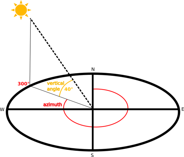
2. The algorithm allows you to specify the position of the light source: Azimuth has values from 0 (North) through 90 (East), 180 (South) and 270 (West), while the Vertical angle sets how high the light source is (0 to 90 degrees).

3. We will use the following values:

   • Z factor at 1.0

   • Azimuth (horizontal angle) at 300.0°

   • Vertical angle at 40.0°

   

4. Save the file in a new folder exercise_data/raster_analysis/ with the name hillshade

5. Finally click on Run

hillshade と呼ばれる新しいレイヤーが次のように表示されます:

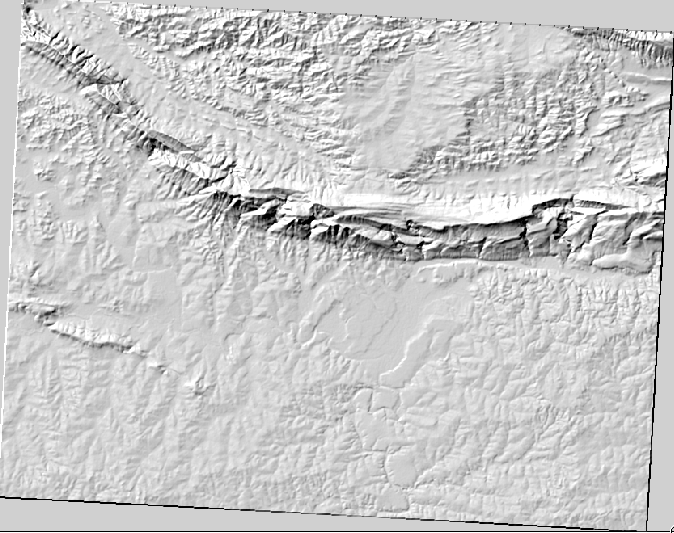
きれいで3次元的に見えますが、これは改善できるでしょうか? 陰影図はそれだけでは石膏模型のように見えます。どうにかしてそれを他のよりカラフルなラスターと一緒に使用できないでしょうか? もちろんできます。オーバーレイとして陰影図を使用します。

7.3.2. Follow Along: 陰影図をオーバーレイとして使用する

陰影図は一日のある時点の日光について非常に有用な情報を提供することができますが審美的な目的で使うこともできます。それを使えば地図をよりよく見せることができます。陰影図をほとんど透過させる設定がその鍵となります。

1. Change the symbology of the original srtm_41_19 layer to use the Pseudocolor scheme as in the previous exercise

2. Hide all the layers except the srtm_41_19 and hillshade layers

3. Click and drag the srtm_41_19 to be beneath the hillshade layer in the Layers panel

4. Set the hillshade layer to be transparent by clicking on the Transparency tab in the layer properties

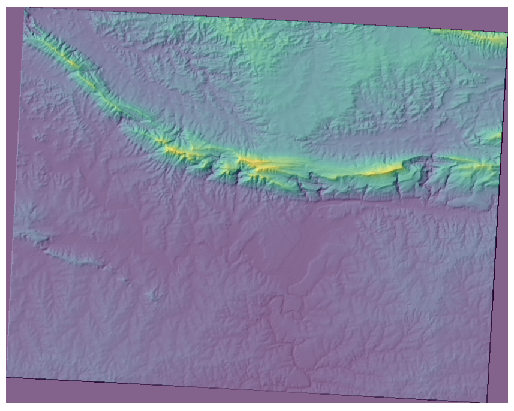
5. 全体の不透明度 を 50% に設定します:

   You'll get a result like this:

   

6. Switch the hillshade layer off and back on in the Layers panel to see the difference it makes.

このように陰影図を使用すると景観の地形を誇張することが可能です。その効果があなたにとって十分な強さだと思えない場合には、 hillshade レイヤーの透明度を変更すればよいですが、もちろん、陰影起伏がより明るくなるほど、その背後の色は薄暗くなります。ちょうど良いバランスを見つける必要があります。

Remember to save the project when you are done.

7.3.3. Follow Along: Finding the best areas

Think back to the estate agent problem, which we last addressed in the Vector Analysis lesson. Let us imagine that the buyers now wish to purchase a building and build a smaller cottage on the property. In the Southern Hemisphere, we know that an ideal plot for development needs to have areas on it that:

• are north-facing

• with a slope of less than 5 degrees

• But if the slope is less than 2 degrees, then the aspect doesn't matter.

Let's find the best areas for them.

7.3.4. Follow Along: 傾斜の計算

Slope informs about how steep the terrain is. If, for example, you want to build houses on the land there, then you need land that is relatively flat.

To calculate the slope, you need to use the Slope algorithm of the Processing ► Raster terrain analysis.

1. Open the algorithm

2. Choose srtm_41_19 as the Elevation layer

3. Keep the Z factor at 1.0

4. Save the output as a file with the name slope in the same folder as the hillshade

5. Click on Run

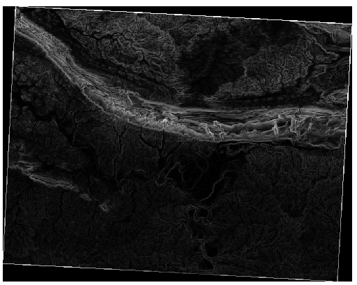
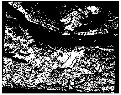
Now you'll see the slope of the terrain, each pixel holding the corresponding slope value. Black pixels show flat terrain and white pixels, steep terrain:

7.3.5. Try Yourself Calculating the aspect

Aspect is the compass direction that the slope of the terrain faces. An aspect of 0 means that the slope is North-facing, 90 East-facing, 180 South-facing, and 270 West-facing.

Since this study is taking place in the Southern Hemisphere, properties should ideally be built on a north-facing slope so that they can remain in the sunlight.

Use the Aspect algorithm of the Processing ► Raster terrain analysis to get the aspect layer saved along with the slope.

結果をチェックする

7.3.6. Follow Along: Finding the north-facing aspect

Now, you have rasters showing you the slope as well as the aspect, but you have no way of knowing where ideal conditions are satisfied at once. How could this analysis be done?

その答えは ラスター計算機 です。

QGIS has different raster calculators available:

• Raster ► Raster Calculator

• In processing:

  • Raster Analysis ► Raster calculator

  • GDAL ► Raster miscellaneous ► Raster calculator

  • SAGA ► Raster calculus ► Raster calculator

Each tool is leading to the same results, but the syntax may be slightly different and the availability of operators may vary.

We will use Raster Analysis ► Raster calculator in the Processing Toolbox

1. Open the tool by double clicking on it.

   • The upper left part of the dialog lists all the loaded raster layers as name@N, where name is the name of the layer and N is the band.

   • In the upper right part you will see a lot of different operators. Stop for a moment to think that a raster is an image. You should see it as a 2D matrix filled with numbers.

2. North is at 0 (zero) degrees, so for the terrain to face north, its aspect needs to be greater than 270 degrees or less than 90 degrees. Therefore the formula is:

   aspect@1 <= 90 OR aspect@1 >= 270
   

3. Now you have to set up the raster details, like the cell size, extent and CRS. This can be done manually or it can be automatically set by choosing a Reference layer. Choose this last option by clicking on the ... button next to the Reference layer(s) parameter.

4. In the dialog, choose the aspect layer, because we want to obtain a layer with the same resolution.

5. Save the layer as aspect_north.

   The dialog should look like:

   

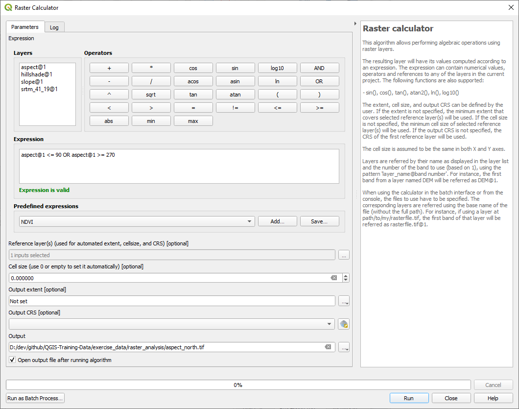
6. Finally click on Run.

あなたの結果はこのようになります:

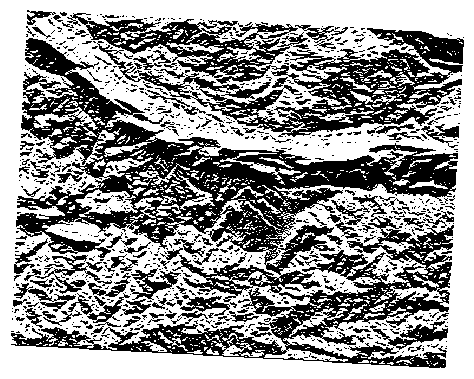
The output values are 0 or 1. What does it mean? For each pixel in the raster, the formula we wrote returns whether it matches the conditions or not. Therefore the final result will be False (0) and True (1).

7.3.7. Try Yourself More criteria

Now that you have done the aspect, create two new layers from the DEM.

• The first shall identify areas where the slope is less than or equal to 2 degrees

• The second is similar, but the slope should be less than or equal to 5 degrees.

• Save them under exercise_data/raster_analysis as slope_lte2.tif and slope_lte5.tif.

結果をチェックする

7.3.8. Follow Along: ラスター分析結果を組み合わせる

Now you have generated three raster layers from the DEM:

• aspect_north: terrain facing north

• slope_lte2: slope equal to or below 2 degrees

• slope_lte5: slope equal to or below 5 degrees

Where the condition is met, the pixel value is 1. Elsewhere, it is 0. Therefore, if you multiply these rasters, the pixels that have a value of 1 for all of them will get a value of 1 (the rest will get 0).

The conditions to be met are:

• at or below 5 degrees of slope, the terrain must face north

• at or below 2 degrees of slope, the direction that the terrain faces does not matter.

Therefore, you need to find areas where the slope is at or below five degrees AND the terrain is facing north, OR the slope is at or below 2 degrees. Such terrain would be suitable for development.

これらの抽出条件を満たすエリアを計算します:

1. Open the Raster calculator again

2. Use this expression in Expression:

   ( aspect_north@1 = 1 AND slope_lte5@1 = 1 ) OR slope_lte2@1 = 1
   

3. Set the Reference layer(s) parameter to aspect_north (it does not matter if you choose another - they have all been calculated from srtm_41_19)

4. Save the output under exercise_data/raster_analysis/ as all_conditions.tif

5. Click Run

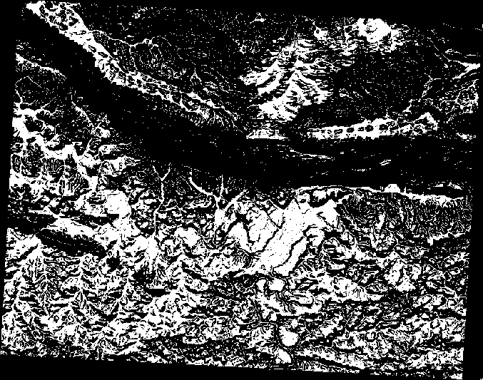
結果：

ヒント

The previous steps could have been simplified using the following command:

((aspect@1 <= 90 OR  aspect@1 >= 270) AND slope@1 <= 5) OR slope@1 <= 2

7.3.9. Follow Along: ラスターを簡素化する

As you can see from the image above, the combined analysis has left us with many, very small areas where the conditions are met (in white). But these aren't really useful for our analysis, since they are too small to build anything on. Let us get rid of all these tiny unusable areas.

1. Open the Sieve tool (GDAL ► Raster Analysis in the Processing Toolbox)

2. Set the Input file to all_conditions, and the Sieved to all_conditions_sieve.tif (under exercise_data/raster_analysis/).

3. Set the Threshold to 8 (minimum eight contiguous pixels), and check Use 8-connectedness.

   

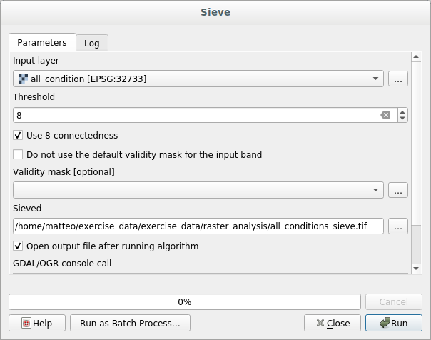
   Once processing is done, the new layer will be loaded.

   

   What is going on? The answer lies in the new raster file's metadata.

4. View the metadata under the Information tab of the Layer Properties dialog. Look the STATISTICS_MINIMUM value: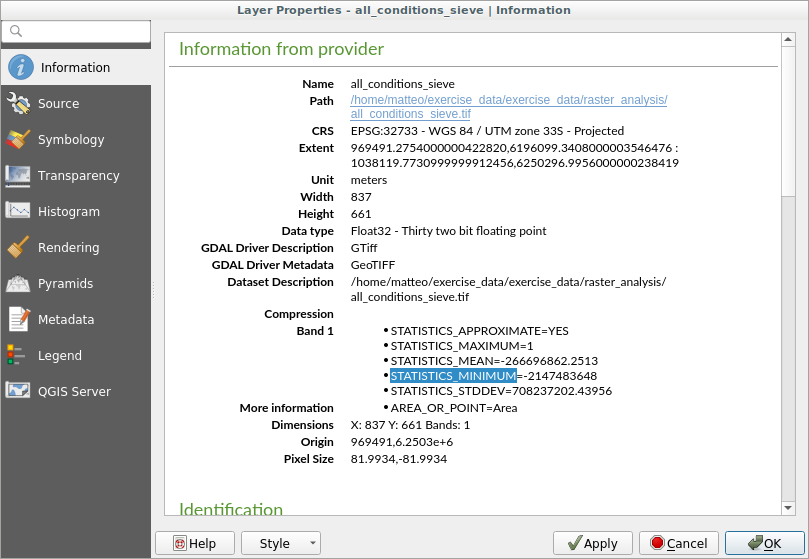

   

   This raster, like the one it is derived from, should only feature the values 1 and 0, but it has also a very large negative number. Investigation of the data shows that this number acts as a null value. Since we are only after areas that weren't filtered out, let us set these null values to zero.

5. Open the Raster Calculator, and build this expression:

   (all_conditions_sieve@1 <= 0) = 0
   

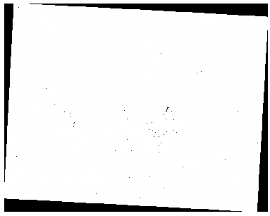
   This will maintain all non-negative values, and set the negative numbers to zero, leaving all the areas with value 1 intact.

6. Save the output under exercise_data/raster_analysis/ as all_conditions_simple.tif.

出力はこのようになります:

これは期待されたもので、以前の結果を簡素化したものです。あなたが得た結果が期待したものでない場合は、メタデータ(および該当する場合はベクターの属性)を見ると問題を解決するための要点がわかることを覚えておいて下さい。

7.3.10. Follow Along: Reclassifying the Raster

We have used the Raster calculator to do calculations on raster layers. There is another powerful tool that we can use to extract information from existing layers.

Back to the aspect layer. We know now that it has numerical values within a range from 0 through 360. What we want to do is to reclassify this layer to other discrete values (from 1 to 4), depending on the aspect:

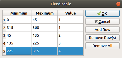
• 1 = North (from 0 to 45 and from 315 to 360);

• 2 = East (from 45 to 135)

• 3 = South (from 135 to 225)

• 4 = West (from 225 to 315)

This operation can be achieved with the raster calculator, but the formula would become very very large.

The alternative tool is the Reclassify by table tool in Raster analysis in the Processing Toolbox.

1. Open the tool

2. Choose aspect as the Input raster layer

3. Click on the ... of Reclassification table. A table-like dialog will pop up, where you can choose the minimum, maximum and new values for each class.

4. Click on the Add row button and add 5 rows. Fill in each row as the following picture and click OK:

   

   The method used by the algorithm to treat the threshold values of each class is defined by the Range boundaries.

5. Save the layer as reclassified.tif in the exercise_data/raster_analysis/ folder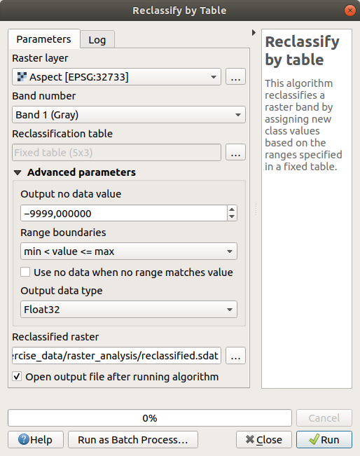

   

6. Click on Run

If you compare the native aspect layer with the reclassified one, there are not big differences. But by looking at the legend, you can see that the values go from 1 to 4.

Let us give this layer a better style.

1. Open the Layer Styling panel

2. Choose Paletted/Unique values, instead of Singleband gray

3. Click on the Classify button to automatically fetch the values and assign them random colors:

   

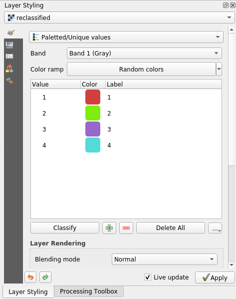
The output should look like this (you can have different colors given that they have been randomly generated):

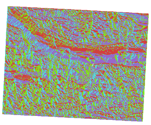
With this reclassification and the paletted style applied to the layer, you can immediately differentiate the aspect areas.

7.3.11. Follow Along: Querying the raster

Unlike vector layers, raster layers don't have an attribute table. Each pixel contains one or more numerical values (singleband or multiband rasters).

All the raster layers we used in this exercise consist of just one band. Depending on the layer, pixel values may represent elevation, aspect or slope values.

How can we query the raster layer to get the value of a pixel? We can use the ^{Identify Features} button!

1. Select the tool from the Attributes toolbar.

2. Click on a random location of the srtm_41_19 layer. Identify Results will appear with the value of the band at the clicked location:

   

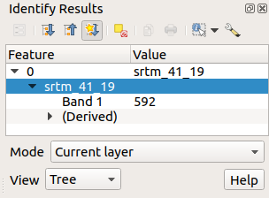
3. You can change the output of the Identify Results panel from the current tree mode to a table one by selecting Table in the View menu at the bottom of the panel: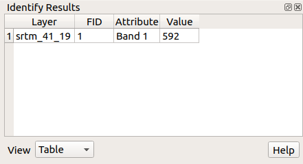

   

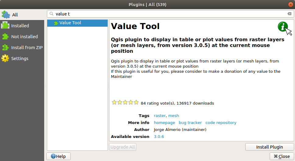
Clicking each pixel to get the value of the raster could become annoying after a while. We can use the Value Tool plugin to solve this problem.

1. Go to Plugins ► Manage/Install Plugins...

2. In the All tab, type value t in the search box

3. Select the Value Tool plugin, press Install Plugin and then Close the dialog.

   

   The new Value Tool panel will appear.

   ちなみに

   If you close the panel you can reopen it by enabling it in the View ► Panels ► Value Tool or by clicking on the icon in the toolbar.

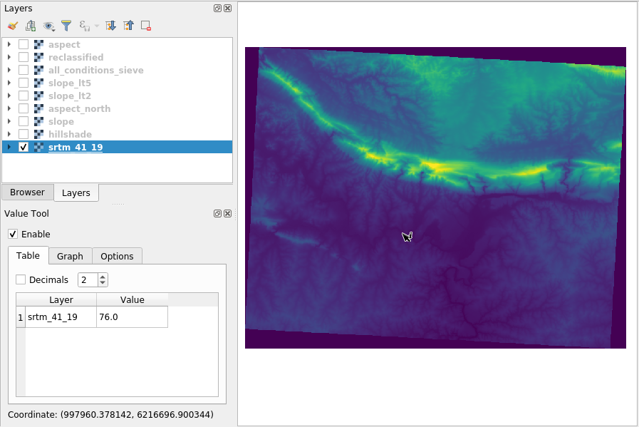
4. To use the plugin just check the Enable checkbox and be sure that the srtm_41_19 layer is active (checked) in the Layers panel.

5. Move the cursor over the map to see the value of the pixels.

   

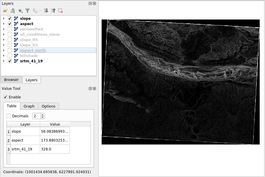
6. But there is more. The Value Tool plugin allows you to query all the active raster layers in the Layers panel. Set the aspect and slope layers active again and hover the mouse on the map:

   

7.3.12. In Conclusion

DEMから様々な種類の分析結果を取り出す方法を見てきました。陰影起伏や傾斜、斜面方位の計算をしました。またこれらの結果をさらに分析し結合するためにラスタ計算機の使用方法を見てきました。最後に、レイヤを再分類する方法と結果をクエリする方法を学びました。

7.3.13. What's Next?

２つの分析結果が得られました：潜在的に適した小地所を示すベクター分析の結果と潜在的に適した地形を示すラスター分析の結果です。この問題の最終的な結果に到達するためにどのようにこれらを組み合わせるか？それが次のレッスンのトピックです。次のモジュールで始まります。