7.3. Lesson: Terrain Analysis
Certain types of rasters allow you to gain more insight into the terrain that they represent. Digital Elevation Models (DEMs) are particularly useful in this regard. In this lesson you will use terrain analysis tools to find out more about the study area for the proposed residential development from earlier.
The goal for this lesson: To use terrain analysis tools to derive more information about the terrain.
7.3.1.  Follow Along: Calculating a Hillshade
We are going to use the same DEM layer as in the previous lesson.
If you are starting this chapter from scratch, use the
Browser panel and load the
raster/SRTM/srtm_41_19.tif.
The DEM layer shows you the elevation of the terrain, but it can sometimes seem a little abstract. It contains all the 3D information about the terrain that you need, but it doesn’t look like a 3D object. To get a better impression of the terrain, it is possible to calculate a hillshade, which is a raster that maps the terrain using light and shadow to create a 3D-looking image.
We are going to use algorithms in the menu.
Click on the menu
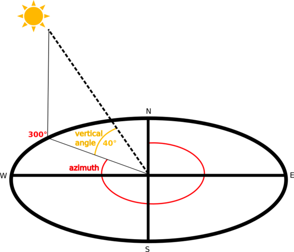
The algorithm allows you to specify the position of the light source: Azimuth has values from 0 (North) through 90 (East), 180 (South) and 270 (West), while the Vertical angle sets how high the light source is (0 to 90 degrees). We will use the default values:
Save the file in a new folder
raster_analysiswithin the folderexercise_datawith the namehillshadeFinally click on Run
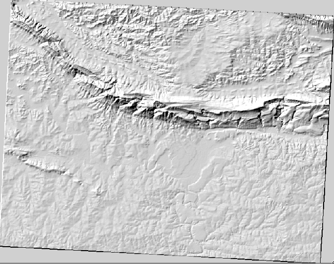
You will now have a new layer called hillshade that looks like this:
That looks nice and 3D, but can we improve on this? On its own, the hillshade looks like a plaster cast. Can’t we use it together with our other, more colorful rasters somehow? Of course we can, by using the hillshade as an overlay.
7.3.2. Follow Along: Using a Hillshade as an Overlay
A hillshade can provide very useful information about the sunlight at a given time of day. But it can also be used for aesthetic purposes, to make the map look better. The key to this is setting the hillshade to being mostly transparent.
Change the symbology of the original srtm_41_19 layer to use the Pseudocolor scheme as in the previous exercise
Hide all the layers except the srtm_41_19 and hillshade layers
Click and drag the srtm_41_19 to be beneath the hillshade layer in the Layers panel
Set the hillshade layer to be transparent by clicking on the Transparency tab in the layer properties
Set the Global opacity to
50%.You’ll get a result like this:
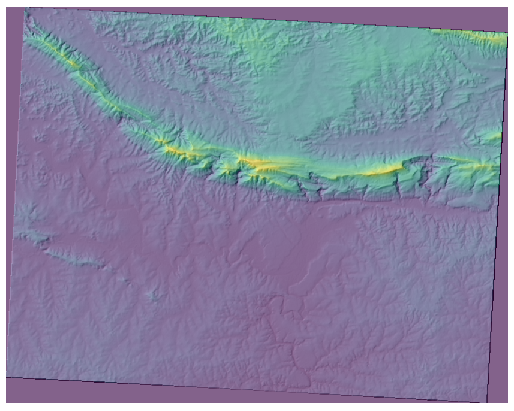
Switch the hillshade layer off and back on in the Layers panel to see the difference it makes.
Using a hillshade in this way, it’s possible to enhance the topography of the landscape. If the effect doesn’t seem strong enough to you, you can change the transparency of the hillshade layer; but of course, the brighter the hillshade becomes, the dimmer the colors behind it will be. You will need to find a balance that works for you.
Remember to save the project when you are done.
7.3.3.  Follow Along: Calculating the Slope
Another useful thing to know about the terrain is how steep it is. If, for example, you want to build houses on the land there, then you need land that is relatively flat.
To do this, you need to use the algorithm of the .
Open the algorithm
Choose srtm_41_19 as the Elevation layer
Save the output as a file with the name
slopein the same folder as thehillshadeClick on Run
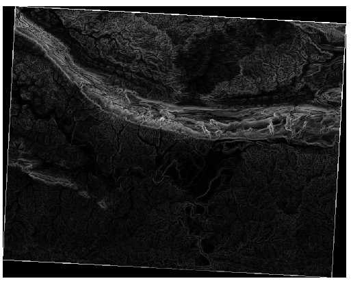
Now you’ll see the slope of the terrain, with black pixels being flat terrain and white pixels, steep terrain:
7.3.4. Try Yourself Calculating the aspect
Aspect is the compass direction that the slope of the terrain faces. An aspect of 0 means that the slope is North-facing, 90 East-facing, 180 South-facing, and 270 West-facing.
Since this study is taking place in the Southern Hemisphere, properties should ideally be built on a north-facing slope so that they can remain in the sunlight.
Use the Aspect algorithm of the to get the layer.
7.3.5. Follow Along: Using the Raster Calculator
Think back to the estate agent problem, which we last addressed in the Vector Analysis lesson. Let us imagine that the buyers now wish to purchase a building and build a smaller cottage on the property. In the Southern Hemisphere, we know that an ideal plot for development needs to have areas on it that are north-facing, and with a slope of less than five degrees. But if the slope is less than 2 degrees, then the aspect doesn’t matter.
Fortunately, you already have rasters showing you the slope as well as the aspect, but you have no way of knowing where both conditions are satisfied at once. How could this analysis be done?
The answer lies with the Raster calculator.
QGIS has different raster calculators available:
In processing:
Each tool is leading to the same results, but the syntax may be slightly different and the availability of operators may vary.
We will use in the Processing Toolbox
Open the tool by double clicking on it.
The upper left part of the dialog lists all the loaded raster layers as
name@N, wherenameis the name of the layer andNis the band.In the upper right part you will see a lot of different operators. Stop for a moment to think that a raster is an image. You should see it as a 2D matrix filled with numbers.
North is at 0 (zero) degrees, so for the terrain to face north, its aspect needs to be greater than 270 degrees and less than 90 degrees. Therefore the formula is:
aspect@1 <= 90 OR aspect@1 >= 270
Now you have to set up the raster details, like the cell size, extent and CRS. This can be done manually or it can be automatically set by choosing a
Reference layer. Choose this last option by clicking on the … button next to the Reference layer(s) parameter.In the dialog, choose the aspect layer, because we want to obtain a layer with the same resolution.
Save the layer as
aspect_north.The dialog should look like:
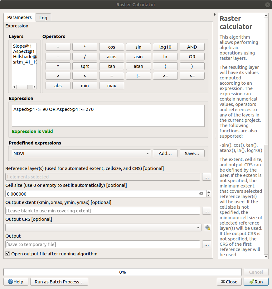
Finally click on Run.
Your result will be this:
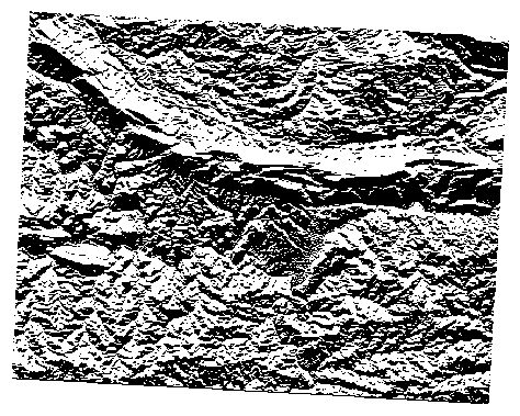
The output values are 0 or 1.
What does it mean?
The formula we wrote contains the conditional operator OR.
Therefore the final result will be False (0) and True (1).
7.3.6. Try Yourself More criteria
Now that you have done the aspect, create two new layers from the DEM.
The first shall identify areas where the slope is less than or equal to
2degreesThe second is similar, but the slope should be less than or equal to
5degrees.Save them under
exercise_data/raster_analysisasslope_lte2.tifandslope_lte5.tif.
7.3.7. Follow Along: Combining Raster Analysis Results
Now you have generated three raster layers from the DEM:
aspect_north: terrain facing north
slope_lte2: slope equal to or below 2 degrees
slope_lte5: slope equal to or below 5 degrees
Where the conditions are met, the pixel value is 1.
Elsewhere, it is 0.
Therefore, if you multiply these rasters, the pixels that have a value
of 1 for all of them will get a value of 1 (the rest will get
0).
The conditions to be met are:
at or below 5 degrees of slope, the terrain must face north
at or below 2 degrees of slope, the direction that the terrain faces does not matter.
Therefore, you need to find areas where the slope is at or below five
degrees AND the terrain is facing north, OR the slope is at or
below 2 degrees. Such terrain would be suitable for development.
To calculate the areas that satisfy these criteria:
Open the Raster calculator again
Use this expression in Expression:
( aspect_north@1 = 1 AND slope_lte5@1 = 1 ) OR slope_lte2@1 = 1
Set the Reference layer(s) parameter to
aspect_north(it does not matter if you choose another - they have all been calculated fromsrtm_41_19)Save the output under
exercise_data/raster_analysis/asall_conditions.tifClick Run
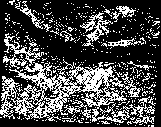
The result:
7.3.8. Follow Along: Simplifying the Raster
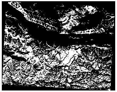
As you can see from the image above, the combined analysis has left us with many, very small areas where the conditions are met. But these aren’t really useful for our analysis, since they are too small to build anything on. Let us get rid of all these tiny unusable areas.
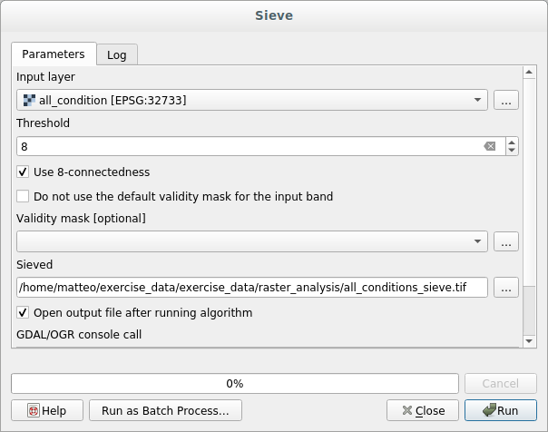
Open the Sieve tool ( in the Processing Toolbox)
Set the Input file to
all_conditions, and the Sieved toall_conditions_sieve.tif(underexercise_data/raster_analysis/).Set the Threshold to 8 (minimum eight contiguous pixels), and check Use 8-connectedness.
Once processing is done, the new layer will be loaded.
What is going on? The answer lies in the new raster file’s metadata.
View the metadata under the Information tab of the Layer Properties dialog. Look the
STATISTICS_MINIMUMvalue: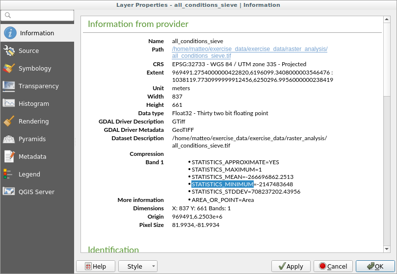
This raster, like the one it is derived from, should only feature the values
1and0, but it has also a very large negative number. Investigation of the data shows that this number acts as a null value. Since we are only after areas that weren’t filtered out, let us set these null values to zero.Open the Raster Calculator, and build this expression:
(all_conditions_sieve@1 <= 0) = 0
This will maintain all non-negative values, and set the negative numbers to zero, leaving all the areas with value
1intact.Save the output under
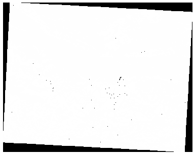
exercise_data/raster_analysis/asall_conditions_simple.tif.
Your output looks like this:
This is what was expected: a simplified version of the earlier results. Remember that if the results you get from a tool aren’t what you expected, viewing the metadata (and vector attributes, if applicable) can prove essential to solving the problem.
7.3.9. Follow Along: Reclassifying the Raster
We have used the Raster calculator to do calculations on raster layers. There is another powerful tool that we can use to extract information from existing layers.
Back to the aspect layer.
We know now that it has numerical values within a range from 0 through
360.
What we want to do is to reclassify this layer to other discrete
values (from 1 to 4), depending on the aspect:
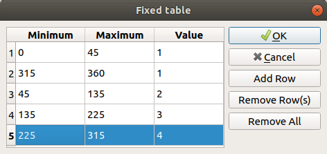
1 = North (from 0 to 45 and from 315 to 360);
2 = East (from 45 to 135)
3 = South (from 135 to 225)
4 = West (from 225 to 315)
This operation can be achieved with the raster calculator, but the formula would become very very large.
The alternative tool is the Reclassify by table tool in in the Processing Toolbox.
Open the tool
Choose aspect as the
Input raster layerClick on the … of Reclassification table. A table-like dialog will pop up, where you can choose the minimum, maximum and new values for each class.
Click on the Add row button and add 5 rows. Fill in each row as the following picture and click OK:
The method used by the algorithm to treat the threshold values of each class is defined by the Range boundaries.
Save the layer as file:reclassified.tif in the
exercise_data/raster_analysis/folder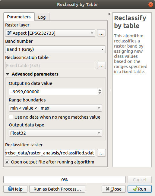
Click on Run
If you compare the native aspect layer with the
reclassified one, there are not big differences.
But by looking at the legend, you can see that the values go from
1 to 4.
Let us give this layer a better style.
Open the Layer Styling panel
Choose Paletted/Unique values, instead of Singleband gray
Click on the Classify button to automatically fetch the values and assign them random colors:
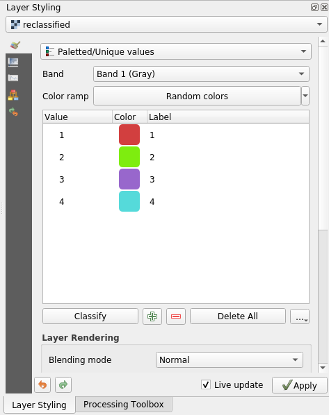
The output should look like this (you can have different colors given that they have been randomly generated):
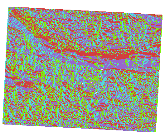
With this reclassification and the paletted style applied to the layer, you can immediately differentiate the aspect areas.
7.3.10. Follow Along: Querying the raster
Unlike vector layers, raster layers don’t have an attribute table. Each pixel contains one or more numerical values (singleband or multiband rasters).
All the raster layers we used in this exercise consist of just one band. Depending on the layer, pixel values may represent elevation, aspect or slope values.
How can we query the raster layer to get the value of a pixel?
We can use the  Identify Features button!
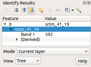
Select the tool from the Attributes toolbar.
Click on a random location of the srtm_41_19 layer. Identify Results will appear with the value of the band at the clicked location:
You can change the output of the Identify Results panel from the current
treemode to atableone by selecting Table in the View menu at the bottom of the panel: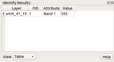
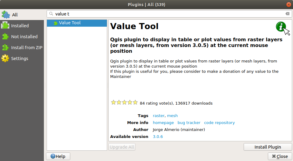
Clicking each pixel to get the value of the raster could become annoying after a while. We can use the Value Tool plugin to solve this problem.
Go to
In the All tab, type
value tin the search boxSelect the Value Tool plugin, press Install Plugin and then Close the dialog.
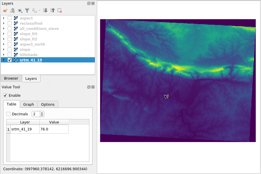
The new Value Tool panel will appear.
Tip
If you close the panel you can reopen it by enabling it in the or by clicking on the icon in the toolbar.
To use the plugin just check the Enable checkbox and be sure that the
srtm_41_19layer is active (checked) in the Layers panel.Move the cursor over the map to see the value of the pixels.
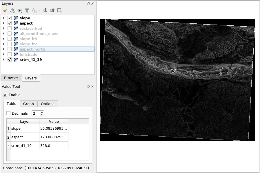
But there is more. The Value Tool plugin allows you to query all the active raster layers in the Layers panel. Set the aspect and slope layers active again and hover the mouse on the map:
7.3.11. In Conclusion
You’ve seen how to derive all kinds of analysis products from a DEM. These include hillshade, slope and aspect calculations. You’ve also seen how to use the raster calculator to further analyze and combine these results. Finally you learned how to reclassify a layer and how to query the results.
7.3.12. What’s Next?
Now you have two analyses: the vector analysis which shows you the potentially suitable plots, and the raster analysis that shows you the potentially suitable terrain. How can these be combined to arrive at a final result for this problem? That’s the topic for the next lesson, starting in the next module.