Kaip dalis atviro kodo programinės įrangos ekosistemos, QGIS sukurta virš įvairių bibliotekų, kurios kartu su savo tiekėjais siūlo galimybes skaityti ir dažnai rašyti daugeliu formatų:
Vektoriniai duomenų formatai, tai GeoPackage, GML, GeoJSON, GPX, KML, kableliais atskirtos reikšmės, ESRI formatai (Shapefile, Geodatabase…), MapInfo ir MicroStation failų formatai, AutoCAD DWG/DXF, GRASS ir daug kitų… Skaitykite pilną palaikomų vektorinių formatų sąrašą.
Rastro duomenų formatai tai GeoTIFF, JPEG, ASCII tinklo XYZ, MBTiles, R ar Idrisi rastrai, GDAL virtualūs, SRTM, Sentinelio duomenys, ERDAS IMAGINE, ArcInfo Binary Grid, ArcInfo ASCII Grid ir daug kitų… Skaitykite pilną palaikomų rastro formatų sąrašą.
Duomenų bazės formatai tai PostgreSQL/PostGIS, SQLite/SpatiaLite, Oracle, MS SQL Server, SAP HANA, MySQL…
Žiniatinklio žemėlapiai ir duomenų paslaugos (WM(T)S, WFS, WCS, CSW, XYZ kaladėlės, ArcGIS paslaugos, …) taipogi palaikomos QGIS tiekėjų. Daugiau informacijos apie kai kuriuos iš jų rasite skyriuje Darbas su OGC / ISO protokolais.
Jūs galite skaityti palaikomus failus iš archyvų aplankų ir naudoti QGIS vidinius formatus, tokius kaip QML failus (QML - The QGIS Style File Format) ir virtualius bei atminties sluoksnius.
GDAL ir vidiniai QGIS tiekėjai palaiko daugiau nei 80 vektorinių ir 140 rastro formatų.
Pastaba
Ne visi išvardinti formatai gali veiktu QGIS dėl įvairių priežasčių. Pavyzdžiui kai kuriems reikia išorinių nuosavybinių bibliotekų ar jūsų OS GDAL/OGR bibliotekų versijos gali nepalaikyti jums reikiamo formato. Norėdami pažiūrėti galimų formatų sąrašą, komandinėje eilutėje paleiskite ogrinfo--formats (vektoriniams) ir gdalinfo--formats (rastrams) arba žiūrėkite QGIS meniu punktą Nustatymai ► Parinktys ► GDAL.
Priklausomai nuo duomenų formato, QGIS yra keli įrankiai, leidžiantis atidaryti duomenų rinkinį, pagrinde juos galima rasti meniu:Sluoksnis –> Pridėti sluoksnį –> ar įrankinėje Tvarkyti sluoksnius (įjungiama per meniu Vaizdas ► Įrankinės). Bet visi šie įrankiai veda į tą patį dialogą: Duomenų šaltinių tvarkyklė, kurį jūs galite atidaryti mygtuku Atverti duomenų šaltinių tvarkyklę, o rasite jį Duomenų šaltinių tvarkymo įrankinėje ar spausdami Ctrl+L. Dialogas Duomenų šaltinių tvarkyklė (Fig. 11.1) teikia bendrą sąsają failais paremtiems duomenimis bei duomenų bazėms ar žiniatinklio paslaugoms, palaikomoms QGIS.
Fig. 11.1 QGIS duomenų šaltinių tvarkyklės dialogas
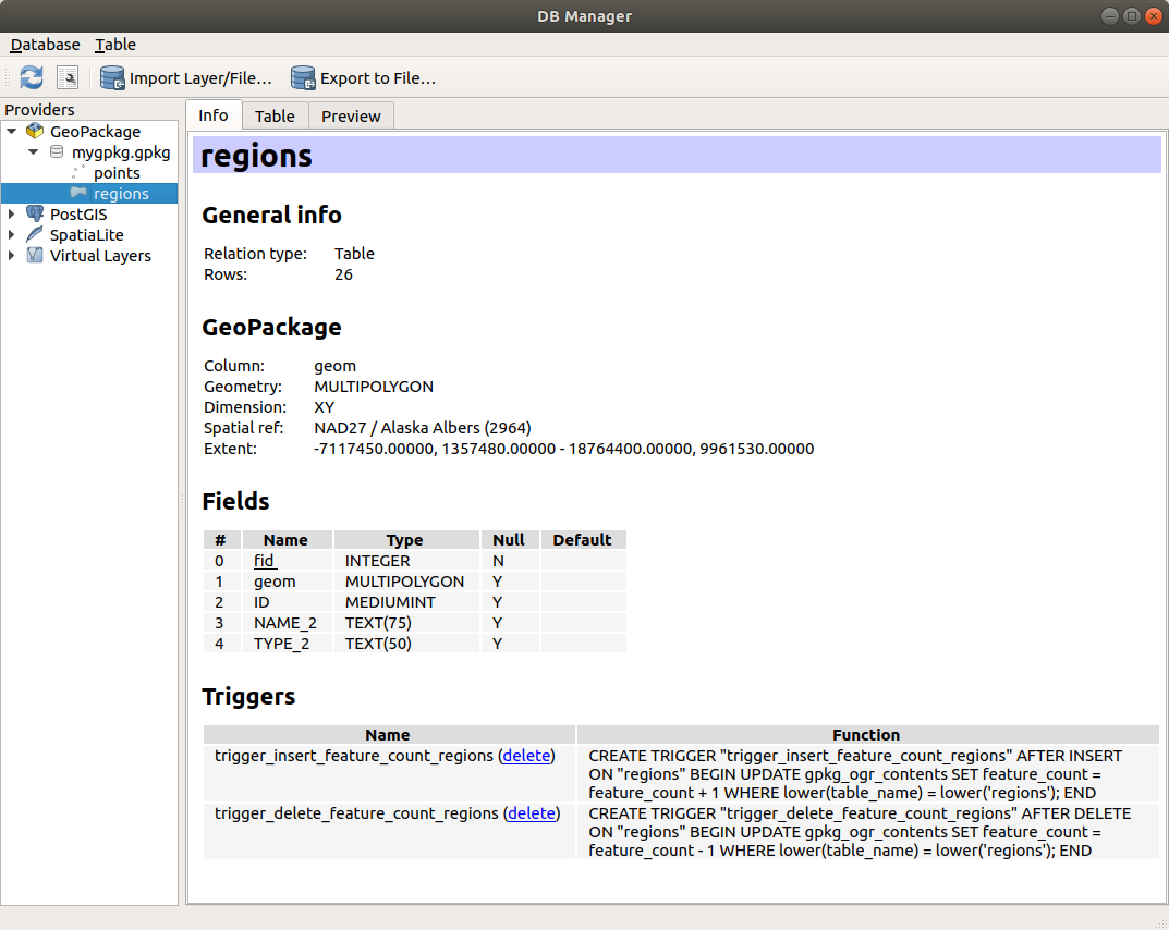
Be šio bendro pradžios taško, dar yra priedas DB tvarkyklė, kuris teikia galimybę analizuoti ir manipuliuoti prijungtas duomenų bazes. Daugiau informacijos apie DB tvarkyklės galimybes rasite skyriuje DB Manager Plugin.
Yra daug kitų įrankių, vidinių ar trečiųjų-šalių priedų, kurie padės jums atverti įvairius duomenų formatus.
Šiame skyriuje aprašomi tik pagal nutylėjimą QGIS esantys duomenų įkėlimo įrankiai. Pagrindinis dėmesys bus skiriamas dialogui Duomenų šaltinių tvarkyklė, bet be visų kortelių aprašymo taipogi bus tyrinėjami įrankiai pagal duomenų tiekėją ar formato specifiką.
Naršyklė - tai vienas iš pagrindinių būdų greitai ir lengvai pridėti duomenis į jūsų projektus. Jis veikia kaip:
Duomenų šaltinių tvarkyklės kortelė, įjungiama paspaudus mygtuką Atverti duomenų šaltinių tvarkyklę (Ctrl+L);
QGIS skydelis, kurį jūs galite atverti per meniu Vaizdas ► Skydeliai (ar Nustatymai ► Skydeliai) arba paspaudę Ctrl+2.
Abiem atvejais Naršyklė padeda jums naršyti po jūsų failų sistemą ir tvarkyti geoduomenis, nepriklausomai nuo sluoksnio tipo (rastras, vektorius, lentelė) ar duomenų šaltinio formato (paprasti ar suspausti failai, duomenų bazės, žiniatinklio šaltiniai).
Naršyklės skydelio viršuje jūs rasite kelis mygtukus, kurie padės jums:
Pridėti parinktus sluoksnius: jūs taipogi galite pridėti duomenis į žemėlapio drobę parinkdami sluoksnio kontekstiniame meniu Pridėti parinktą sluoksnį(ius);
Atnaujinti naršyklės medį;
Filtruoti naršyklę konkrečių duomenų paieškai. Įveskite paieškos žodį ar šabloną ir naršyklė filtruos medį, kad rodytų tik kelius į atitinkamas DB lenteles, failų pavadinimus ar aplankus – kiti duomenys ir aplankai nebus rodomi. Žiūrėkite naršyklės skydelio(2) pavyzdį Fig. 11.2. Lyginimą galima daryti atsižvelgiant į raidžių dydį arba ne. Jį taipogi galima nustatyti į:
Normalų: rodyti elementus, kuriuose yra ieškomas tekstas
Įjungti/išjungti savybių valdiklį: įjungus, naujas valdiklis pridedamas skydelio apačioje ir, kai galima, rodo parinkto elemento metaduomenis.
Skydelio Naršyklė įrašai išdėlioti pagal hierarchiją ir yra keli aukščiausio lygio įrašai:
Parankiniai, kur jūs galite padėti dažnai naudojamas vietas
Erdvinės žymelės, kur jūs galite laikyti dažnai naudojamas žemėlapio apimtis (žr. Žemėlapio apimčių žymelės)
Projekto namai: greitai prieigai prie aplanko, kuriame laikoma (dauguma) su projektų susijusių duomenų. Numatytoji reikšmė yra aplankas, kuriame yra projekto failas.
Namų aplankas failų sistemoje ir failų sistemos šakninis aplankas.
Prijungti vietiniai ar tinklo įrenginiai
Toliau išvardinti keli konteinerių / duomenų bazių tipai ir paslaugų protokolai, priklausomai nuo jūsų platformos ir turimų bibliotekų:
Naršyklė palaiko pertempimą ir numetimą naršyklės viduje, iš naršyklės į drobę ir Sluoksnių skydelį bei iš Sluoksnių skydelio į sluoksnių konteinerius (pvz. GeoPackage) naršyklėje.
Projekto failo elementus naršyklėje galima išplėsti, rodant pilną projekto sluoksnių medį (įskaitant grupes). Projekto elementai veikia taip pat, kaip bet koks kitas naršyklės elementas, taigi juos galima tempti ir numesti naršyklės viduje (pavyzdžiui kopijuoti sluoksnio elementą į geopackage failą) ar pridėti į dabartinį projektą pertempiant ir numetant ar du kartus paspaudus.
Naršyklės skydelio elemento kontekstinis meniu atidaromas paspaudus ant jo dešinį pelės mygtuką.
Failų sistemos aplankų įrašams, kontekstinis meniu leidžia:
Naujas ► sukurti parinktame elemente:
Aplanką…
GeoPackage…
ShapeFile…
Pridėti kaip parankinį: parankinius aplankus galima bet kokiu metu pervadinti (Pervadinti parankinį…) ar išimti (Išimti parankinį).
Slėpti nuo naršyklės: paslėptus failus galima pakeisti į matomus naudojant nustatymą Nustatymai ► Parinktys ► Duomenų šaltiniai ► Paslėpti naršyklės keliai
Greitai skenuoti šį aplanką
Atverti aplanką
Atverti terminale
Savybės…
Aplanko savybės…
Vaikiniams įrašams, kurie yra projektų sluoksniai, kontekstiniame meniu bus palaikantys įrašai. Pavyzdžiui, ne duomenų bazės, ne vektorinių, rastro ar duomenų tinklelio paslaugų įrašai turės:
Eksportuoti sluoksnį ► Į failą…
Pridėti sluoksnį į projektą
Sluoksnio savybės
Atverti su duomenų šaltinių tvarkykle…
Tvarkyti ► Pervadinti „<name of file>“… ar Trinti „<name of file>“…
Rodyti failuose
Failo savybės
Įraše Sluoksnio savybės jūs rasite (panašiai, kaip ir vektorinių ir rastro sluoksnių savybėse, kai sluoksniai pridedami į projektą):
Sluoksnio Metaduomenis. Metaduomenų grupes: Tiekėjo informacija (jei įmanoma, Kelias bus hipernuoroda į šaltinį), Identifikacija, Apimtis, Prieiga, Laukai (vektoriniams sluoksniams), Juostos (rastro sluoksniams), Kontaktai, Jungtys (vektoriniams sluoksniams), Nuorodos (rastro sluoksniams), Istorija.
Peržiūros skydelį
Vektorinių šaltinių atributų lentelę (skydelyje Atributai).
Naudokite Atverti su duomenų šaltinių tvarkykle…, kad tiesiogiai atidarytumėte ir konfigūruotumėte duomenų šaltinį su Duomenų šaltinių tvarkykle naudojant jūsų duomenų šaltinio URI. Tai supaprastina sluoksnio pridėjimo iš Naršyklės procesą leidžiant jums nustatyti konkrečias duomenų šaltinio atidarymo parinktis. Šiuo metu tai veikia su vektoriniais (įskaitant tam skirtus GeoPackage įrašus), rastro ir SpatiaLite duomenų šaltiniais.
Norėdami pridėti į projektą sluoksnį naudojant Naršyklę:
Įjunkite Naršyklę, kaip aprašyta aukščiau. Bus parodytas jūsų failų sistemos, duomenų bazių ir žiniatinklio paslaugų medis. Jums gali prireikti prijungti duomenų bazes ir žiniatinklio paslaugas, kad jos pasirodytų (žr. tam skirtas skiltis).
Raskite sluoksnį sąraše.
Naudokite kontekstinį meniu, du kartus paspauskite pavadinimą arba pertempkite ir numeskite jį į žemėlapio drobę. Jūsų sluoksnis dabar pridėtas į Sluoksnių skydelį ir galite jį matyti žemėlapio drobėje.
Patarimas
Atverkite QGIS projektą tiesiai iš naršyklės
Jūs galite atverti QGIS projektą tiesiai iš Naršyklės skydelio du kartus paspaudę jo pavadinimą arba nutempę ir numetę jį į žemėlapio drobę.
Įkėlus failą jūs galite naršyti po jį naudodami žemėlapio navigacijos įrankius. Norėdami pakeisti sluoksnio stilių, atverkite dialogą Sluoksnio savybės du kartus paspaudę sluoksnio pavadinimą ar paspaudę dešinį pelės mygtuką ant pavadinimo legendoje ir kontekstiniame meniu parinkę Savybės. Daugiau informacijos apie vektorinių sluoksnių simbologijos nustatymus rasite skyriuje Symbology Properties.
Dešinys pelės paspaudimas naršyklės medyje padeda jums:
failui ar lentelei - rodyti jo metaduomenis ar atverti jį jūsų projekte. Lenteles galima pervadinti, trinti ar ištuštinti.
aplankui - jį pasidėti į parankinius ar paslėpti naršyklės medyje. Paslėptus aplankus galima valdyti kortelėje Nustatymai ► Parinktys ► Duomenų šaltiniai.
valdyti jūsų erdvines žymeles: žymeles galima kurti, eksportuoti ir importuoti kaip XML failus.
kurti jungtį su duomenų baze ar žiniatinklio paslauga.
atnaujinti, pervadinti ar ištrinti schemą.
Jūs taipogi galite importuoti failus į duomenų bazes ar kopijuoti lenteles iš vienos schemos/duomenų bazės į kitą naudojant paprastą pertempimą ir numetimą. Galima naudoti antrą naršyklės skydelį, kad pertempimo metu nereikėtų toli sukti slankiklio. Tiesiog pažymėkite failą ir pertempkite bei numeskite jį į kitą skydelį.
Fig. 11.2 QGIS naršyklės skydeliai vienas greta kito
Patarimas
Pridėkite sluoksnius į QGIS tiesiog pertempdami juos iš jūsų OS failų naršyklės
Jūs taipogi galite pridėti failą(us) į projektą tempdami ir numesdami juos iš jūsų operacinės sistemos failų naršyklės į Sluoksnių skydelį ar žemėlapio drobę.
Priedas DB tvarkyklė yra dar vienas įrankis, QGIS palaikomų erdvinių duomenų bazių formatų integravimui ir tvarkymui (PostGIS, SpatiaLite, GeoPackage, Oracle Spatial, MS SQL Server, Virtualūs sluoksniai). Jį galima aktyvuoti per meniu Priedai ► Tvarkyti ir įdiegti priedus….
DB tvarkyklės priedas teikia kelias savybes:
prisijungimas prie duomenų bazių ir jų struktūros bei turinio peržiūra
duomenų bazių lentelių peržiūra
sluoksnių pridėjimas į žemėlapio drobę dvigubu paspaudimu arba tempimu ir numetimu.
sluoksnių pridėjimas į duomenų bazę iš QGIS naršyklės ar kitos duomenų bazės
SQL užklausų kūrimas ir jų išvesties pridėjimas į žemėlapio drobę
Be naršyklės skydelio ir DB tvarkyklės - pagrindinių QGIS teikiamų sluoksnių pridėjimo įrankių, jūs taipogi rasite įrankius, kurie yra naudojami tik su konkrečiais duomenų tiekėjais.
Pastaba
Kai kurie išoriniai priedai taipogi teikia įrankius, skirtus atidaryti QGIS konkrečių formatų failus.
Atidarykite sluoksnių tipo kortelę dialoge Duomenų šaltinių tvarkyklė, t.y. spauskite mygtuką Atverti duomenų šaltinių tvarkyklę (arba spauskite Ctrl+L) ir įjunkite paskirties kortelę, arba:
vektoriniams duomenims (tokiems kaip GML, ESRI Shapefile, Mapinfo ir DXF sluoksniams): spauskite Ctrl+Shift+V, parinkite meniu Sluoksnis ► Pridėti sluoksnį ►Pridėti vektorinį sluoksnį arba spauskite įrankinės mygtuką Pridėti vektorinį sluoksnį.
Fig. 11.4 Vektorinio sluoksnio pridėjimo dialogas
rastro duomenims (tokiems kaip GeoTiff, MBTiles, GRIdded Binary ir DWG sluoksniams): spauskite Ctrl+Shift+R, parinkite meniu Sluoksnis ► Pridėti sluoksnį ►Pridėti rastro sluoksnį arba spauskite įrankinės mygtuką Pridėti rastro sluoksnį.
Naviguokite failų sistemoje ir įkelkite palaikomą duomenų šaltinį. Vienu metu galima įkelti daugiau nei vieną sluoksnį laikant Ctrl kai spaudžiama ant elementų dialoge arba laikant paspaustą Shift, kad parinktumėte diapazoną elementų paspaudus ant pirmo ir tada paskutinio diapazono elemento. Formatų filtre rodomi tik tie formatai, kurie buvo gerai išbandyti. Kitus formatus galima įkelti parinkus Visifailai (viršutinis iškrentančio meniu elementas).
Spauskite Atidaryti, kad įkeltumėte parinktą failą į Duomenų šaltinių tvarkymo dialogą.
Priklausomai nuo parinkto sluoksnio tipo, konfigūravimui bus prieinami papildomos Parinktys (koduotė, geometrijos tipas, lentelės filtravimas, failų rakinimas, duomenų formatavimas …). Šios parinktys detaliai aprašomos konkrečiuose GDAL vektorių ar rastro tvarkyklių dokumentacijose. Parinkčių viršuje esantis hypertekstas jus nuves tiesiai į parinkto failo formato atitinkamos tvarkyklės dokumentaciją.
Fig. 11.6 Shape failo įkėlimas su atvertomis parinktimis
Spauskite Pridėti, kad įkeltumėte failą į QGIS ir parodytumėte jį žemėlapio vaizde. Kai pridedamos vektorinės duomenų aibės su keliais sluoksniais, bus rodomas dialogas Parinkite pridedamus elementus. Šiame dialoge jūs galite parinkti konkrečius jūsų duomenų rinkinio sluoksnius, kuriuos norite pridėti. Taipogi skiltyje Parinktys jūs galite pasirinkti:
Pridėti sluoksnius į grupę
Rodyti sistemines ir vidines lenteles
Rodyti tuščius vektorinius sluoksnius.
Fig. 11.7 matomas QGIS po failo alaska.shp įkėlimo.
Kadangi kai kurie formatai, tokie kaip MapInfo (pvz., .tab) ar Autocad (.dxf) leidžia viename faile kartu laikyti skirtingų tipų geometrijas, įkeliant tokius duomenų rinkinius atidaromas dialogas, kur reikia parinkti geometrijas kiekvienam sluoksniui.
Kortelės Pridėti vektorinį sluoksnį ir Pridėti rastro sluoksnį leidžia įkelti sluoksnius iš šaltini tipų, kitokių nei Failas:
Jūs galite įkelti specifinius vektorinius formatus, tokius kaip ArcInfodvejetainispadengimas, UK.Nacionalinisperdavimoformatas bei pradinį TIGER formatą iš USCensusBureau ar OpenfileGDB. Norėdami tai padaryti, parinkite Aplanką kaip Šaltinio tipą. Tokiu atveju, kai paspausite …Naršyti, galėsite dialoge parinkti aplanką.
Su šaltinio tipu Duomenų bazė jūs galite parinkti esamą duomenų bazės jungtį ar sukurti parinkto tipo naują. Kelios galimos duomenų bazės yra ODBC, EsriPersonalGeodatabase, MSSQLServer kaip ir PostgreSQL ar MySQL .
Paspaudus mygtuką Naujas, atveriamas dialogas Kurti naują OGR duomenų bazės jungtį su parametrais, kuriuos galite rasti skyriuje Įrašytos jungties kūrimas. Paspaudę Atverti jūs parenkate iš galimų lentelių, pavyzdžiui iš duomenų bazių su PostGIS.
:guilabel:`Protokolas: HTTP(S), debesies ir panašiems šaltinių tipams atidaro duomenis, kurie saugomi vietoje arba tinkle, kur jie arba viešai prieinami, arba teikiami privačiuose komercinių debesų saugyklų paslaugomis. Palaikomi protokolų tipai yra:
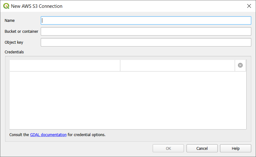
Debesų saugyklos, tokios kaip AWSS3, GoogleCloudStorage, MicrosoftAzureBlob, MicrosoftAzureDataLakeStorage, AlibabaOSSCloud ir OpenStackSwiftStorage, palaiko tiesioginį valdymą per VSI Prisijungimo parinktis, kai pridedami OGR vektorių ar GDAL rastro sluoksniai. Jums reikia iš pradžių užpildyti Kibirėlį ar konteinerį ir Objektų raktą. Tada jūs galite pridėti reikiamą Prisijungimo informaciją.
Pridedant OGR vektorinius ar GDAL rastro sluoksnius per debesimis paremtus protokolus, jūs taipogi galite nurodyti papildomas Prisijungimo parinktis konkrečiai tvarkyklei ar kibirėliui. Kai prisijungimo duomenys randami sluoksnio URI, jie nustatomi automatiškai. Tai leidžia skirtingiems sluoksniams naudoti skirtingus prisijungimo duomenis.
paslauga, palaikanti OGC WFS3 (vis dar eksperimentinis), naudojant GeoJSON ar GEOJSON-atskirtanaujomiseilutėmis formatą ar paremtą CouchDB duomenų baze. Privaloma nurodyti URI, galima nurodyti ir autentifikaciją.
Visiems vektoriniams šaltinių tipams galima nurodyti Koduotę arba naudoti nustatymą Automatinis ►.
Šaltinio tipas OGC API leidžia pasiekti vektorinius ir rastro duomenis iš serverių, kurie įgyvendina OGC API standartus. Norėdami naudoti šią parinktį:
Dialoge Duomenų šaltinių tvarkyklė parinkite OGC API.
Įveskite OGC API paslaugos prieigos tašką, prie kurio norite prisijungti. Pastebėtina, kad nurodant prieigos tašką nereikia jam pridėti priešdėlio „OGCAPI:“.
Spauskite Prisijungti, kad sukurtumėte jungtį su serveriu.
Tinklelis yra nestruktūrinis tinklas, paprastai su laiko ar kitais komponentais. Erdviniame komponente yra aibė viršūnių, kraštinių ir plokštumų 2D ir 3D erdvėje. Daugiau informacijos apie tinklelio sluoksnius rasite skyriuje Darbas su tinklelio duomenimis.
Norėdami pridėti tinklelio sluoksnį į QGIS:
Atverkite dialogą Duomenų šaltinių tvarkyklė arba parenkant jį per meniu Sluoksnis ►, arba paspaudus mygtuką Atverti duomenų šaltinių tvarkyklę.
Kairiame skydelyje įjunkite kortelę Tinklelis
Spauskite mygtuką …Naršyti, kad parinktumėte failą. Palaikomi Įvairūs formatai.
Parinkite failą ir spauskite Pridėti. Sluoksnis bus pridėtas naudojant savą tinklelio braižymą.
Jei parinktame faile yra daug tinklelių sluoksnių, tada jums bus parodytas dialogas, kuriame jūsų paprašys pasirinkti įkeliamus posluoksnius. Pasirinkite ir spauskite Gerai, tada sluoksniai bus įkelti su savo tinklelio braižymu. Taipogi galima įkelti juos grupėje.
Fig. 11.8 Tinklelio kortelė Duomenų šaltinių tvarkyklėje
Atskirus failus (pvz. .txt, .csv, .dat, .wkt) galima įkelti naudojant aukščiau aprašytus įrankius. Tokiu būdu jie bus rodomi kaip paprastos lentelės. Kartais atskirtuose teksto failuose gali būti koordinatės / geometrijos, kurias jūs galite norėti pavaizduoti. Tam ir sukurta galimybė Pridėti atskirtą teksto sluoksnį.
Spauskite piktogramą Atverti duomenų šaltinių tvarkyklę, kad atvertumėte Duomenų šaltinių tvarkyklės dialogą
Įjunkite kortelę Atskirtas tekstas
Parinkite importuojamą atskirto teksto failą (pvz., qgis_sample_data/csv/elevp.csv) paspausdami mygtuką …Naršyti.
Lauke Sluoksnio pavadinimas pateikite pavadinimą, kurį reikia projekte naudoti kaip sluoksnio pavadinimą (pvz. Aukštis).
Sukonfigūruokite nustatymus, kad jie atitiktų jūsų duomenų aibės poreikius, kaip paaiškinta žemiau.
Parinkus failą QGIS bando išnagrinėti failą su paskutiniu naudotu skirtuku, identifikuojant laukus ir eilutes. Kad QGIS galėtų teisingai išnagrinėti failą, labai svarbu parinkti teisingą skirtuką. Jūs galite nurodyti skirtuką pasirinkdami vieną iš:
CSV (kableliu atskirtos reikšmės) kad naudotumėte kablelio simbolį.
Reguliarios išraiškos skirtukas ir įveskite tekstą į lauką Išraiška. Pavyzdžiui jei norite pakeisti skirtuką į tabuliacijos simbolį, naudokite \t (tai reguliariose išraiškose naudojama kaip tabuliacijos simbolis).
Savi skirtukai, pasirinkite iš iš anksto apibrėžtų skirtukų, tokių kaip kablelis, tarpas, tabuliacija, kabliataškis, … .
Duomenų atpažinimui galima naudoti keletą kitų patogių parinkčių:
Skaičius išmetamų antraštės eilučių: patogu, kai norite išvengti kelių pirmų failo eilučių importo metu, nes arba jos yra tuščios, arba jose yra kitoks formatavimas.
Pirmame įraše yra laukų pavadinimai: pirmos eilutės reikšmės yra naudojamos laukų pavadinimams, kitu atveju QGIS naudoja laukų pavadinimus field_1, field_2…
Atpažinti laukų tipus: automatiškai atpažįsta lauko tipą. Išjungus šią parinktį visi atributai laiko tekstiniais.
Trupmeninės dalies skirtukas yra kablelis: galite priversti naudoti kablelį kaip trupmeninės dalies skirtuką.
Apkarpyti laukus: leidžia jums apkarpyti laukus ir gale esančius tarpus.
Išmesti tuščius laukus.
Savos loginės reikšmės: leidžia jums pridėti savo eilučių porą, kuri bus aptinkama kaip loginės reikšmės.
QGIS bando automatiškai aptikti laukų tipus (nebent varnelė Aptikti laukų tipus yra išjungta) tiriant papildomo CSVT failo turinį (žr. GeoCSV specifikacija) ir skenuojant visą failą, kad būtų įsitikinta, kad reikšmes tikrai galima konvertuoti be klaidų, atsarginis lauko tipas yra tekstas.
Aptiktas lauko tipas matosi po lauko pavadinimu pavyzdinių duomenų peržiūros lentelėje ir, jei reikia, jį galima pakeisti rankomis.
Palaikomi šie laukų tipai:
Loginis nuo raidžių dydžio nepriklausančios tekstinės poros, kurios interpretuojamos kaip loginės reikšmės, yra 1/0, true/false, t/f, yes/no
Sveikasskaičius(integer)
Sveikasskaičius(integer-64bit)
Dešimtainisskaičius: dvigubo tikslumo slankaus kablelio skaičius
Išnagrinėjus failą, nustatykite Geometrijos apibrėžimą kaip
Taško koordinates ir pateikite X lauką, Y lauką, Z lauką (3-matmenų duomenims) ir M lauką (matavimo matmeniui), jei sluoksnis yra taško geometrijos ir turi tokius laukus. Jei koordinatės nurodytos laipsniais/minutėmis/sekundėmis, įjunkite varnelę DMS koordinatės. Pateikite atitinkamą Geometrijos CRS naudojant valdiklį Parinkti CRS.
Gerai žinomo teksto (WKT) parinktį, jei erdvinė informacija išreikšta kaip WKT: parinkite Geometrijos lauką, kuriame yra WKT geometrija ir parinkite atitinkamą Geometrijos tipą arba leiskite QGIS jį aptikti automatiškai. Pateikite atitinkamą Geometrijos CRS naudojant valdiklį Parinkti CRS.
Jei faile yra neerdviniai duomenys, įjunkite Nėra geometrijos (lentelėje tik atributai) ir jis bus įkeltas kaip paprasta lentelė.
Naudoti erdvinį indeksą, kad pagerintumėte erdvinių geoobjektų rodymo ir parinkimo greitaveiką.
Naudoti poaibio indeksą, kad pagerintumėte poaibių filtrų greitaveiką (kai jie apibrėžti sluoksnio savybėse).
Stebėti failą, kad būtų stebima, kada failą keičia kitos programos kol veikia QGIS.
Tada spauskite Pridėti, kad pridėtumėte sluoksnį į žemėlapį. Mūsų pavyzdyje į projektą pridedamas taškų sluoksnis vardu Elevation ir jis elgiasi lygiai taip pat, kaip visi kiti QGIS žemėlapio sluoksniai. Šis sluoksnis yra šaltinio failo .csv užklausos rezultatas (taigi su juo susijęs) ir jį reikės įrašyti, jei norėsite gauti erdvinį sluoksnį diske.
DXF ir DWG failus galima pridėti į QGIS tiesiog pertempus juos iš Naršyklės skydelio. Jūsų paprašys parinkti posluoksnius, kuriuos norite pridėti į projektą. Sluoksniai pridedami su atsitiktinėmis stiliaus savybėmis.
Pastaba
DXF failams su keliais geometrijos tipais (taškas, linija ir/arba poligonas), sluoksniai bus pavadinti kaip <failas.dxf> esybės <geometry type>.
Kad išlaikytumėte dxf/dwg failo struktūrą ir jo simbologiją QGIS’e, jūs galite naudoti tam skirtą įrankį Projektas ► Importuoti/Eksportuoti ► Importuoti sluoksnius iš DWG/DXF…, kuris leis jums:
importuoti elementus iš brėžinio failo į GeoPackage duomenų bazę.
pridėti importuotus elementus į projektą.
Dialoge DWG/DXF importas, norėdami importuoti brėžinio failo turinį:
Įveskite Šaltinio brėžinio vietą, t.y. DWG/DXF brėžinio failą, kurį reikia importuoti.
Nurodykite brėžinio failo duomenų koordinačių atskaitos sistemą.
Įveskite Paskirties paketo vietą, t.y. GeoPackage failą, į kurį bus įrašyti duomenys. Jei nurodomas esamas failas, jis bus perrašytas.
Parinkite, kaip importuoti blokus:
Išskleisti blokų geometrijas: importuoja brėžinio failo blokus kaip normalius elementus.
Išskleisti bloko geometrijas ir pridėti įterpimo taškus: importuoja brėžinio failo blokus kaip normalius elementus ir prideda įterpimo tašką kaip taškų sluoksnį.
Tik pridėti taškus: prideda blokų įterpimo tašką kaip taškų sluoksnį.
Įjunkite Naudoti kreives, kad keistumėte importuojamus sluoksnius į kreivių geometrijos tipą.
Naudokite mygtuką Importuoti, kad importuotumėte brėžinį į paskirties GeoPackage failą. GeoPackage duomenų bazė bus automatiškai užpildyta brėžinio failo turiniu. Priklausomai nuo failo dydžio, tai gali užtrukti.
Po to, kai .dwg ar .dxf duomenys importuojami į GeoPackage duomenų bazę, apatinėje dialogo dalyje esanti dalis užpildoma importuoto failo sluoksniais. Ten jūs galite pasirinkti ir pridėti sluoksnius į QGIS projektą:
Viršuje nurodykite Grupės pavadinimą, kad grupuotumėte brėžinių failus projekte. Pagal nutylėjimą ji nustatoma pagal šaltinio brėžinio failą.
Įjunkite rodomus sluoksnius: kiekvienas parinktas sluoksnis pridedamas į ad hoc grupę, kurioje yra brėžinio sluoksnio taškų, užrašų, linijų ir plotų geoobjektai. Sluoksnių stiliai panašūs į tuos, kurie buvo *CAD.
Parinkite ar sluoksnis turi būti matomas atidarant.
Įjungus parinktį Sulieti sluoksnius, visi sluoksniai bus vienoje grupėje.
OpenStreetMap projektas yra populiarus, nes daugumoje šalių negalima nemokamai gauti geoduomenų, tokių kaip kelių žemėlapiai. OSM projekto tikslas yra sukurti laisvą redaguojamą pasaulio žemėlapį naudojant GPS duomenis, oro fotografijas ir vietines žinias. Kad padėtų šiam tikslui, QGIS teikia OSM duomenų palaikymą.
Naudojant Naršyklės skydelį jūs galite įsikelti .osm failą į žemėlapio drobę, tokiu atveju jums bus parodytas dialogas, kuriame galėsite pasirinkti posluoksnius pagal geometrijos tipą. Įkeltuose sluoksniuose bus visi to geometrijos tipo duomenys iš .osm failo ir jie išlaikys osm failo duomenų struktūrą.
Kai pirmą kartą įkeliate duomenis iš SpatiaLite duomenų bazės, pradėkite:
spausdami įrankinės mygtuką the Pridėti SpatiaLite sluoksnį
parinkdami Pridėti SpatiaLite sluoksnį… iš meniu Sluoksniai ► Pridėti sluoksnį
ar spausdami Ctrl+Shift+L
Tai pakels langą, kuris leis jums arba prisijungti prie QGIS jau žinomos duomenų bazės (kurią jūs pasirinktumėte iškrentančiame meniu) arba apibrėšite naują jungtį į naują duomenų bazę. Kad apibrėžtumėte naują jungtį, spauskite Nauja ir naudokite failų naršyklę, kad parodytumėte, kur yra jūsų SpatiaLite duomenų bazę, kuri yra failas su plėtiniu .sqlite.
QGIS taipogi leidžia redaguojamus SpatiaLite vaizdus.
Yra daug failų formatų, leidžiančių laikyti GPS duomenis. QGIS naudoja formatą, vadinamą GPX (GPS eXchange format), kuris yra standartinis apsikeitimo formatas, kuriame gali būti bet koks skaičius taškų, maršrutų ir pėdsakų viename faile.
Naudokite mygtuką …Naršyti, kad parinktumėte GPX failą, tada naudokite varneles, kad parinktumėte geoobjektų tipus, kuriuos norite įkelti iš to GPS failo. Kiekvienas geoobjektų tipas bus įkeltas kaip atskiras sluoksnis.
Norint skaityti ir rašyti QGIS palaikomų duomenų bazių formatų lenteles, jums reikia sukurti jungti į tą duomenų bazę. Nors QGIS naršyklės skydelis yra paprasčiausias ir rekomenduojamas būdas prisijungti ir naudoti duomenų bazes, QGIS teikia ir kitus įrankius prisijungimui ir jų lentelių įkėlimui:
Pridėti PostGIS sluoksnį… ar paspaudus Ctrl+Shift+D
Pridėti MS SQL Server sluoksnį
Pridėti Oracle Spatial sluoksnį… ar paspaudus Ctrl+Shift+O
Pridėti SAP HANA Spatial sluoksnį… ar paspaudus Ctrl+Shift+G
Šie įrankiai pasiekiami per Sluoksnių tvarkymo įrankinę ir meniu Sluoksnis ► Pridėti sluoksnį ►. Prisijungimas prie SpatiaLite duomenų bazės aprašytas skyriuje SpatiaLite sluoksniai.
Patarimas
Sukurkite jungtį į duomenų bazę QGIS naršyklės skydelyje
Parinkite naršyklės medyje atitinkamą duomenų bazės formatą, spauskite dešinį pelės mygtuką ir parinkite prisijungimą, tai pateiks jums prisijungimo prie duomenų bazės dialogą.
Dauguma prisijungimo dialogų turi bendrą struktūrą:
skiltis su prisijungimo prie duomenų bazės informacija
skiltis su parinktimis, nurodančiomis kurių duomenų galima prašyti iš duomenų bazės
Kai pirmą kartą naudojate PostGIS duomenų šaltinį, jūs turite sukurti jungtį į duomenų bazę, kurioje yra duomenys. Spauskite atitinkamą mygtuką, kaip parodyta aukščiau, atidarius kortelę PostgreSQL dialoge Duomenų šaltinių tvarkyklė. Kad pasiektumėte jungčių tvarkyklę, spauskite mygtuką Naujas, bus parodytas dialogas Sukurti naują PostGIS jungtį.
Fig. 11.12 Naujos PostGIS jungties kūrimo dialogas
Pavadinimas: Šios jungties pavadinimas. Jis gali būti toks pat kaip Duomenų bazė.
Paslauga: Paslaugos parametras, kurį galima naudoti kaip alternatyvą mašinai/prievadui (ir potencialiai duomenų bazei). Jis gali būti apibrėžtas faile pg_service.conf. Daugiau informacijos rasite skyriuje PostgreSQL paslaugos jungties failas.
Stotis: Duomenų bazės mašinos pavadinimas. Jis turi galėti išsispręsti ir tikti atverti TCP/IP jungtį ar nusiųsti patikrinimo signalą į serverį. Jei duomenų bazė yra tame pačiame kompiuteryje kaip QGIS, tiesiog įveskite localhost.
Prievadas: PostgreSQL duomenų bazės prievadas, kuriuo ji klausosi. Numatytasis PostGIS prievadas yra 5432.
Duomenų bazė: Duomenų bazės pavadinimas.
SSL režimas: SSL šifravimo režimas. Galimos šios parinktys:
Pirmenybė (numatytoji): Man šifravimas nesvarbus, bet aš sutinku gaišti papildomą laiką šifravimui, jei serveris jį palaiko.
Reikalauti: Aš noriu, kad mano duomenys būtų užšifruoti ir aš sutinku su papildomai gaištamu laiku. Aš tikiu, kad tinklas užtikrins, kad aš visada prisijungiu prie to serverio, prie kurio noriu.
Tikrinti CA: Aš noriu, kad mano duomenys būtų šifruoti ir sutinku su papildomu reikiamu laiku. Aš noriu būti tikras, kad jungiuosi prie serverio, kuriuo pasitikiu.
Tikrinti pilnai: Aš noriu, kad mano duomenys būtų šifruoti ir sutinku su papildomu reikiamu laiku. Aš noriu būti tikras, kad jungiuosi prie serverio, kuriuo pasitikiu ir jis yra tas, kurį aš nurodžiau.
Leisti: Man saugumas nesvarbu, bet aš mokėsiu kainą už papildomą šifravimo darbą, jei serveris to reikalauja.
Išjungti: Man saugumas nesvarbus ir aš nenoriu gaišti papildomo laiko šifravimui.
Sesijos rolė: naudojama nustatant dabartinės sesijos dabartinio naudotojo identifikatorių. Tai naudinga, kai reikia automatiškai duoti naujo objekto (lentelės, vaizdo, funkcijos) nuosavybę sesijos rolės grupei ir tokiu būdu dalinti susijusiomis teisėmis su visais sesijos rolės grupės nariais. Daugiau apie tai skaitykite <https://www.postgresql.org/docs/current/sql-set-role.html>`_.
Autentifikacija, paprasta.
Naudotojo vardas: Prisijungimui prie duomenų bazės naudojamas vardas.
Slaptažodis: Prisijungimui prie duomenų bazės naudotoju Naudotojas slaptažodis.
Jūs galite įrašyti bet kurį ar abu parametrus - Naudotojovardą ir Slaptažodį, tokiu atveju jie bus naudojami pagal nutylėjimą kiekvieną kartą, kai jums reikės prisijungti prie šios duomenų bazės. Jei jų neįrašysite, jums reikės juos įvesti jungiantis prie duomenų bazės kitose QGIS sesijose. Jūsų įvesti prisijungimo parametrai laikomi laikiname vidiniame podėlyje ir grąžinami, kai prireikia tos pačios duomenų bazės naudotojo/slaptažodžio, kol jūs baigiate dabartinę QGIS sesiją.
Įspėjimas
QGIS naudotojo nustatymai ir saugumas
Kortelėje Autentifikacija išsaugojus naudotoją ir slaptažodį neapsaugoti prisijungimo duomenys bus laikomi jungties konfigūracijoje. Šie prisijungimo duomenys bus matomi jei, pavyzdžiui, pasidalinsite projektu su kuo nors kitu. Taigi patariama vietoje to įrašyti jūsų prisijungimo duomenis į Autentifikacijos konfigūraciją, (kortelė Konfigūracijos - daugiau informacijos rasite skyriuje Autentifikacijos sistema) arba paslaugos jungties faile (pavyzdį rasite PostgreSQL paslaugos jungties failas).
Pasirinktinai, priklausomai nuo duomenų bazės tipo, jūs galite įjungti šias varneles:
Rodyti tik sluoksnius sluoksnių registruose
Nespręsti neribotų stulpelių tipų (GEOMETRY)
Žiūrėti tik schemoje „public“
Rodyti ir lenteles be geometrijos: nurodo, kad pagal nutylėjimą reikia rodyti ir lenteles, kurios neturi geometrijos.
Naudoti įvertintus lentelės metaduomenis: Inicializuojant sluoksnius, gali prireikti įvairių užklausų, kad būtų sužinotos duomenų bazės lentelėje saugomų geometrijų charakteristikos. Įjungus šią parinktį šios užklausos tiria tik dalį eilučių ir naudoja lentelės statistiką, o ne visą lentelę. Tai gali drastiškai pagreitinti veiksmus su dideliais duomenų rinkiniais, bet gali reikšti neteisingą sluoksnių charakteristiką (pvz. gali būti neteisingai nustatytas filtruotų sluoksnių geoobjektų skaičius) ir gali net sukelti keistą elgseną, jei stulpeliuose, kuriuose turėtų būti unikalios reikšmės, iš tikrųjų taip nėra.
Leisti įrašyti/įkelti QGIS projektus duomenų bazėje - daugiau informacijos čia
Leisti įrašyti/įkelti QGIS sluoksnių metaduomenis duomenų bazėje - daugiau informacijos čia
Nustačius visus parametrus ir parinktis galite patikrinti jungtį paspausdami mygtuką Bandyti jungtį arba pritaikyti spausdami mygtuką Gerai.
Paslaugos jungties failas leidžia PostgreSQL jungties parametrus susieti su vienu paslaugos pavadinimu. Tokį paslaugos pavadinimą gali būti nurodyti klientas ir bus naudojami susiję nustatymai.
Jis vadinasi .pg_service.conf *nix sistemose (GNU/Linux, macOS etc.) ir pg_service.conf Windows.
Aukščiau pateiktame pavyzdyje yra dvi paslaugos: water_service ir wastewater_service. Jūs galite jas naudodami prisijungdami iš QGIS, pgAdmin ir t.t. nurodydami tik paslaugos, prie kurios norite prisijungti, pavadinimą (be skliaustelių). Jei norite naudoti paslaugą su psql, galite tai padaryti taip psqlservice=water_service.
Jei nenorite įrašyti slaptažodžių į paslaugos failą, taipogi galite naudoti variantą .pg_pass.
Pastaba
QGIS Serveris ir paslauga
Kai naudojamas paslaugų failas ir QGIS Serveris, jūs privalote sukonfigūruoti paslaugą ir serverio pusėje. Galite laikytis instrukcijų, pateiktų QGIS Serverio dokumentacijoje.
*nix operacinėse sistemose (GNU/Linux, macOS etc.) jūs galite įrašyti .pg_service.conf failą į naudotojų namų aplanką ir PostgreSQL klientai į jį automatiškai atsižvelgs. Pavyzdžiui, jei prisijungęs naudotojas yra web, .pg_service.conf reikia įrašyti į aplanką /home/web/, kad jis veiktų (nenurodant jokių aplinkos kintamųjų).
Jūs galite nurodyti paslaugos failo vietą sukurdami aplinkos kintamąjį PGSERVICEFILE (pvz. įvykdykite komandą exportPGSERVICEFILE=/home/web/.pg_service.conf jūsų *nix OS, kad laikinai nustatytumėte kintamąjį PGSERVICEFILE).
Jūs taipogi galite padaryti paslaugų failą prieinamu visai sistemai (visiems naudotojams) arba padėdami .pg_service.conf failą į pg_config--sysconfdir arba pridėdami aplinkos kintamąjį PGSYSCONFDIR, kad nurodytumėte aplanką, kuriame yra paslaugos failas. Jei paslauga su tokiu pačiu pavadinimu apibrėžta ir naudotojo, ir sistemos faile, bus naudojamas naudotojo failas.
Įspėjimas
Naudojant Windows yra keli įspėjimai:
Paslaugos failą reikia įrašyti kaip pg_service.conf, o ne .pg_service.conf.
Paslaugos failą reikia įrašyti Unix formatu, kad jis veiktų. Tai galima padaryti pavyzdžiui atidarius jį su Notepad++ ir parinkus Edit ► EOL Conversion ► UNIX Format ► File save.
Jūs galite pridėti aplinkos kintamuosius keliais būdais. Patikrintas būdas, kuris užtikrintai veikia, yra Control Panel ► System and Security ► System ► Advanced system settings ► Environment Variables pridėti PGSERVICEFILE su keliu - pvz. C:\Users\John\pg_service.conf
Pridėjus aplinkos kintamąjį jums gali tekti iš naujo paleisti jūsų kompiuterį.
Oracle Spatial erdvinės savybės padeda naudotojams valdyti geografinius ir vietos duomenis naudojant savus tipus Oracle duomenų bazėje. Šis jungties dialogas siūlo:
Duomenų bazė: Oracle egzemplioriaus SID ar SERVICE_NAME;
Prievadas: Prievado numeris, kuriuo klausosi Oracle duomenų bazė. Numatytasis prievadas yra 1521;
Parinktys: specifinės Oracle jungties parinktys (pvz. OCI_ATTR_PREFETCH_ROWS, OCI_ATTR_PREFETCH_MEMORY). Parinkčių eilutės formatas yra kabliataškiais atskirtas sąrašas parinkčių pavadinimų ar porų parinktis=reikšmė;
Darbo erdvė: Darbo erdvė, į kurią reikia persijungti;
Schema: Schema, kurioje laikomi duomenys
Pasirinktinai galite įjungti šias varneles:
Ieškoti tik metaduomenų lentelėje: rodo tik tas lenteles, kurios yra vaizde all_sdo_geom_metadata. Tai gali pagreitinti pradinį erdvinių lentelių parodymą.
Ieškoti tik naudotojo lentelėse: ieškant erdvinių lentelių apsiribojama tik lentelėmis, kurių savininkas yra dabartinis naudotojas.
Rodyti ir lenteles be geometrijos: nurodo, kad pagal nutylėjimą reikia rodyti ir lenteles, kurios neturi geometrijos.
Naudoti įvertintas lentelių statistikas sluoksnių metaduomenims: kai ruošiamas sluoksnis, reikia turėti įvairius Oracle lentelės metaduomenis, tokius kaip lentelės įrašų skaičius, geometrijos tipas, geometrijos stulpelių duomenų erdvinė apimtis. Jei lentelėje yra daug įrašų, šių rodiklių nustatymas gali užtrukti daug laiko. Įjungus šią parinktį bus vykdomi šie greiti metaduomenų nustatymo veiksmai: įrašų skaičius nustatomas pagal all_tables.num_rows. Lentelės apimtis visada nustatoma naudojant funkciją SDO_TUNE.EXTENTS_OF, net jei taikomas sluoksnio filtras. Lentelės geometrija nustatoma pagal pirmus 100 ne null geometrijos įrašų.
Tik esami geometrijos tipai: rodo tik esamos geometrijos tipus ir nesiūlo pridėti kitų.
Įtraukti papildomus geometrijos atributus.
Leisti įrašyti/įkelti QGIS projektus duomenų bazėje - daugiau informacijos čia
Schema: Leidžia nurodyti vieną schemą, kuria apsiriboti prisijungiant. Jei ji nurodyta, naršyklės skydelyje ir duomenų šaltinio pasirinkime jungtyje bus rodomos lentelės iš atitinkančios schemos. Tai galima naudoti ribojant duombazės darbą, kurio prireiks pildant jungties lenteles, kai kalba apie dideles duomenų bazių saugyklas.
Patarimas
Oracle Spatial sluoksniai
Paprastai Oracle Spatial sluoksnis apibrėžiamas įrašu lentelėje USER_SDO_METADATA.
Kad įsitikintumėte, kad parinkimo įrankiai veikia korektiškai, rekomenduojama, kad jūsų lentelės turėtų pirminį raktą.
Norėdami sukurti naują MS SQL Server jungtį jūs turite pateikti toliau išvardintą informaciją Jungties detalių dialoge:
Jungties pavadinimas
Tiekėjas/DSN
Mašina
Prisijungimo informacija. Jūs galite pasirinkti Įrašyti jūsų prisijungimo duomenis.
Nueikite į skiltį Duomenų bazės detalės ir spauskite mygtuką Duomenų bazių sąrašas, kad peržiūrėtumėte pasiekiamus duomenų rinkinius. Parinkite duomenų rinkinius, kurių jums reikia, tada spauskite Gerai. Pasirinktinai jūs galite vykdyti Bandyti jungtį. Paspaudus Gerai, dialogas Kurti naują MS SQL Server jungtį užsidarys, Duomenų šaltinių tvarkyklėje spauskite Prisijungti, parinkite sluoksnį ir spauskite Pridėti.
Pasirinktinai galite įjungti šias parinktis:
Ieškoti tik metaduomenų lentelėje geometry_columns: skenuojant rodo tik tas lentas, kurios yra metaduomenų lentelėje geometry_columns. Tai gali pagreitinti lentelių skenavimą.
Naudoti sluoksnio apimtį iš lentelės geometry_columns: ši parinktis, priklausanti nuo ankstesnės, leidžia QGIS praleisti apimties skaičiavimą įkeliant sluoksnius, taip sumažinant įkrovimui reikiamą laiką. Remiamasi rankiniu būdu nurodyta apimtimi naudojant QGIS-specifinius laukus (qgis_xmin, qgis_xmax, qgis_ymin, qgis_ymax) lentelėje geometry_columns.
Naudoti pirminį raktą iš lentelės geometry_columns: leidžia QGIS praleisti pirminio rakto skaičiavimą įkeliant vaizdus, taip sumažinant įkėlimui reikiamą laiką. Jis remiasi rankiniu vardų užpildymu QGIS-specifiniame qgis_pkey stulpelyje lentelėje geometry_columns. Jei pirminiam raktui naudojamas daugiau nei vienas stulpelis, jie turėtų būti užpildyti kaip kableliais atskirtos reikšmės.
Taipogi rodyti lenteles be geometrijos: lentelės be prisegto geometrijos lauko irgi bus rodomos galimų lentelių sąraše.
Naudoti įvertintus lentelės parametrus: bus naudojami tik įvertinti lentelės metaduomenys. Taip išvengiama lėtų lentelės skenavimų, bet dėl to gali būti gautos netikslios sluoksnio savybės, tokios kaip sluoksnio apimtis.
Praleisti netinkamų geometrijų apdorojimą: visas įrašų su netinkamomis geometrijomis apdorojimas bus išjungtas. Tai pagreitina tiekėją, bet bet kokios lentelėje esančios netinkamos geometrijos reikš neprognozuojamus ir kartais trūkstamus įrašus. Įjunkite šią parinktį tik kai esate įsitikinę, kad visos duomenų bazėje esančios geometrijos yra tinkamos ir bet kokios naujai pridėtos geometrijos ar lentelės taipogi bus tinkamos.
Naudoti tik schemų poaibį leis jums filtruoti MS SQL jungties schemas. Įjungus šią parinktį bus rodomos tik pažymėtos schemos. Jūs galite spausti Įjungti ar Išjungti bet kurią sąraše esančią schemą.
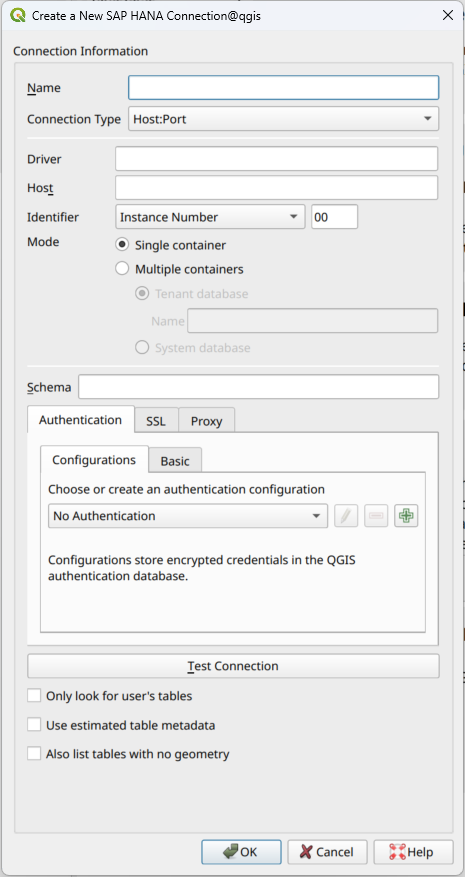
Jei norite prisijungti prie SAP HANA duomenų bazės, jums reikia SAP HANA kliento. Atsisiųsti SAP HANA klientą jūsų platformai galite iš SAP vystymo įrankių svetainės.
Fig. 11.14 Naujos SAP HANA jungties kūrimo dialogas
Galima įvesti šiuos parametrus:
Pavadinimas: šios jungties pavadinimas.
Tvarkyklė: HANA ODBC tvarkyklės pavadinimas. Jis yra HDBODBC, jei naudojate 64-bitų QGIS, HDBODBC32, jei naudojate 32-bitų QGIS. Atitinkamas tvarkyklės pavadinimas įvedamas automatiškai.
Tvarkyklė: arba pavadinimas, kuriuo buvo registruota SAP HANA ODBC tvarkyklė /etc/odbcinst.ini, arba pilnas kelias iki SAP HANA ODBC tvarkyklės. Pagal nutylėjimą SAP HANA kliento diegyklė įdiegs ODBC tvarkyklę į /usr/sap/hdbclient/libodbcHDB.so.
Serveris: Duomenų bazės serverio pavadinimas.
Identifikatorius: identifikuoja serverio egzempliorių, prie kurio reikia prisijungti. Tai gali būti Egzemplioriaus numeris ar Prievado numeris. Egzemplioriaus numerį sudaro du skaitmenys, prievadai yra intervale nuo 1 iki 65,535.
Režimas: nurodo kokiu režimu veikia SAP HANA egzempliorius. Šis nustatymas naudojamas tik tada, jei paskyros Identifikatorius nurodytas Egzemplioriaus numeris. Jei duomenų bazėje yra keli konteineriai, jūs galite arba prisijungti prie nuomininko su vardu, nurodytu Nuomininko duomenų bazė, arba galite prisijungti prie sisteminės duomenų bazės.
Schema: šis parametras nėra privalomas. Jei nurodyta schema, QGIS duomenų ieškos tik toje schemoje. Jei šis laukas bus paliktas tuščias, QGIS duomenų ieškos visose schemose.
Autentifikacija ► Bazinė.
Naudotojo vardas: prisijungimo prie duomenų bazės naudotojo vardas.
Slaptažodis: prisijungimo prie duomenų bazės slaptažodis.
Tiekėjas: nurodo kriptografinės bibliotekos tiekėją, kurį naudoja SSL komunikacija. sapcrypto turėtų veikti visose platformose, openssl turėtų veikti , mscrypto turėtų veikti ir commoncrypto reikalauja, kad būtų įdiegtas CommonCryptoLib.
Tikrinti SSL sertifikatą: įjungus šią parinktį, SSL sertifikatas bus tikrinamas naudojant pasitikėjimo saugyklą, kuri nurodyta Pasitikėjimo saugojimo faile su viešu raktu.
Permušti mašinos pavadinimą sertifikate: nurodo mašinos pavadinimą, kurį reikia naudoti tikrinant serverio identitetą. Čia nurodytas mašinos vardas tikrina serverio identitetą, o ne mašinos pavadinimą, kuriuo jungtis buvo sukurta. Jei jūs kaip mašinos pavadinimą nurodysite *, tada serverio mašinos pavadinimas nebus tikrinamas. Kiti pakeitimo ženklai neleidžiami.
Raktų saugyklos failas su privačiu raktu: šiuo metu ignoruojama. Šis parametras galėtų ateityje leisti autentifikuotis naudojant sertifikatą vietoje naudotojo vardo ir slaptažodžio.
Pasitikėjimo saugyklos failas su viešu raktu: nurodo kelią iki pasitikėjimo saugyklos failo, kuriame yra serverio vieši sertifikatai, jei naudojama OpenSSL. Paprastai pasitikėjimo saugykloje yra šakninis sertifikatas arba sertifikatas įstaigos, kuri pasirašė serverio viešus sertifikatus. Jei jūs naudojate kriptografijos biblioteką CommonCryptoLib ar msCrypto, tada palikite šią parinktį tuščią.
Žiūrėti tik naudotojo lentelėse: įjungus šią parinktį QGIS ieškos tik lentelių ir vaizdų, kurių savininkas yra naudotojas, kuris jungiasi prie duomenų bazės.
Naudoti įvertintus lentelės metaduomenis: įjungus šią parinktį, bus naudojami įvertinti lentelės metaduomenys, jei jie yra surinkti. Didelėms lentelėms taip išvengiama lėto lentelės įkėlimo ir potencialiai brangių skaičiavimų, bet gali reikšti neteisingas sluoksnio savybes, tokias kaip sluoksnio apimtis. Greitas apimties įvertinimas galimas pradedant QRC1/2024 ir SP8 su HANA Cloud ir atitinkamai HANA vietiniame.
Taipogi rodyti lenteles be geometrijų: įjungus šią parinktį QGIS ieško ir lentelių bei vaizdų, kuriuose nėra erdvinių stulpelių.
Patarimas
Prisijungimas prie SAP HANA debesies
Jei norite prisijungti prie SAP HANA debesies egzemplioriaus, jums paprastai reikia nurodyti Prievado numerį443 ir įjungti parinktį Įjungti TLS/SSL šifravimą.
Kai turite apsibrėžę vieną ar daugiau jungčių į duomenų baze (žr. skiltį Įrašytos jungties kūrimas), jūs galite iš jų įkelti sluoksnius. Žinoma, tam reikia, kad duomenys būtų pasiekiami. Daugiau informacijos apie tai, kaip įkelti duomenis į PostGIS duomenų bazę rasite skiltyje Importing Data into PostgreSQL.
Kad įkeltumėte sluoksnį iš duomenų bazės, jums reikia įvykdyti šiuos žingsnius:
Atidarykite atitinkamos duomenų bazės kortelę dialoge Duomenų šaltinių tvarkyklė.
Iškrentančiame sąraše parinkite jungties pavadinimą ir spauskite Prisijungti.
Įjunkite ar įjunkite parinktį Taipogi rodyti lenteles be geometrijos.
Pasirinktinai naudokite kelias Paieškos parinktis, kad sutrumpintumėte lentelių sąrašą iki to, kuris atitinka jūsų kriterijus. Jūs taipogi galite nurodyti šią parinktį prieš paspaudžiant mygtuką Prisijungti, kad pagreitintumėte informacijos ištraukimą iš duomenų bazės.
Prieinamų sluoksnių sąraše suraskite sluoksnį(ius), kurį norite pridėti.
Parinkite jį paspaudimu. Jūs galite parinkti kelis sluoksnius, parinkdami laikydami mygtuką Shift ar Ctrl.
Jei taikoma, naudokite mygtuką Nustatyti filtrą (ar du kartus spauskite sluoksnį), kad įjungtumėte dialogą Užklausos kūrėjas (žr. skiltį Query Builder) ir nurodykite, kuriuos geoobjektus reikia įkelti iš parinkto sluoksnio. Filtro išraiška bus rodoma stulpelyje sql. Šį apribojimą galima išimti ar keisti Sluoksnio savybės ► Bendra ► Tiekėjo geoobjektų filtras.
Varnelė stulpelyje Parinktipagalid, kuri pagal nutylėjimą įjungta, ištraukia geoobjektų id be jų atributų, todėl dažniausiai pagreitina duomenų įkėlimą.
Spauskite mygtuką Pridėti, kad pridėtumėte sluoksnį į žemėlapį.
Naudokite naršyklės skydelį, kad pagreitintumėte duomenų bazės lentelės(ių) įkėlimą
DB lentelių pridėjimas naudojant Duomenų šaltinių tvarkyklę kartais gali užimti daug laiko, nes QGIS kiekvienai lentelei iš karto ištraukia statistikas ir savybes (pvz. geometrijos tipą ir lauką, CRS, geoobjektų skaičių). Kad to išvengtumėte, kai jungtis nustatyta, geriau naudoti Naršyklės skydelį ar DB tvarkyklę, kad temptumėte ir numestumėte duomenų bazės lenteles į žemėlapio drobę.
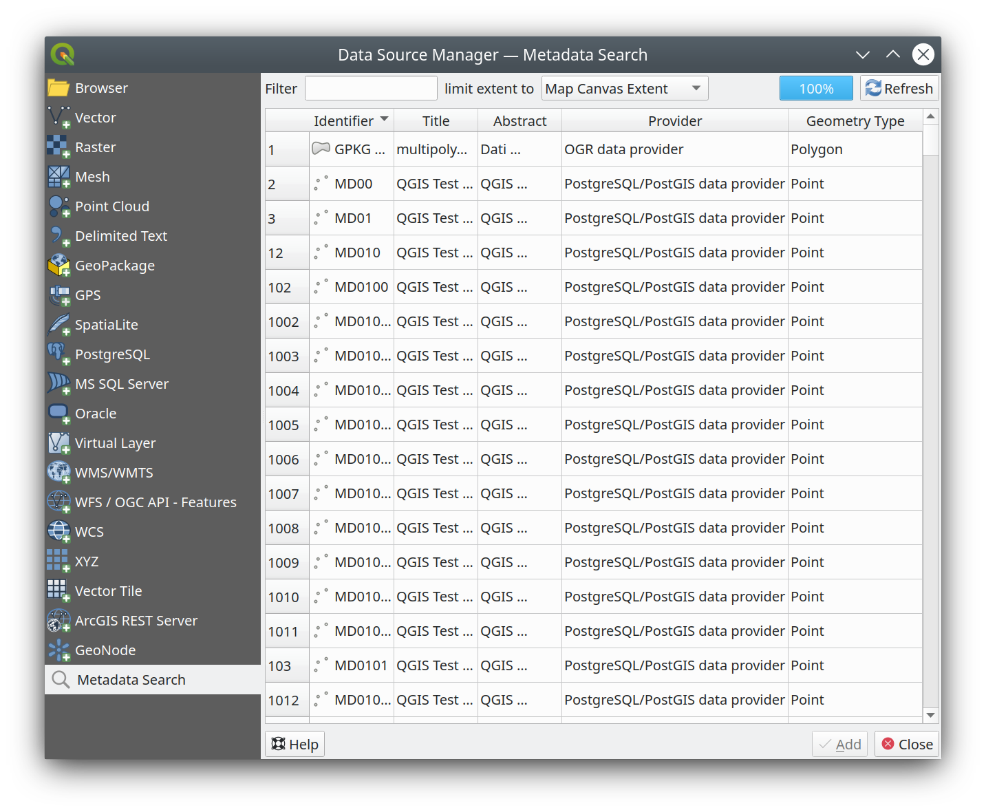
Pagal nutylėjimą QGIS gali gauti sluoksnio metaduomenis iš jungties ar duomenų tiekėjų, kurie leidžia saugoti metaduomenis (daugiau informacijos rasite metaduomenų įrašymas į duomenų bazę). Skydelis Metaduomenų paieška leidžia naršyti po sluoksnius pagal jų metaduomenis ir pridėti juos į projektą (arba du kartus paspaudus arba naudojant mygtuką Pridėti). Sąrašą galima filtruoti:
pagal tekstą, stebint metaduomenų savybių aibę (identifikatorių, pavadinimą, santrauką)
pagal erdvinę apimtį, naudojant dabartinio projekto apimtį arba žemėlapio drobės apimtį
pagal sluoksnio (geometrijos) tipą
Pastaba
Metaduomenų šaltinis įgyvendinamas per sluoksnio metaduomenų tiekėjo sistemą, kurią gali išplėsti priedai.
Fig. 11.16 Sluoksnio metaduomenų paieškos skydelis
Laikinas juodraštinis sluoksnis: atminties sluoksnis, kuris susietas su projektu (daugiau informacijos rasite skyriuje Creating a new Temporary Scratch Layer)
Virtualūs sluoksniai: sluoksnis, kuris gaunamas įvykdžius kito sluoksnio(ių) užklausą (daugiau informacijos rasite skyriuje Creating virtual layers)
Sluoksnio apibrėžimus galima įrašyti kaip Sluoksnio apibrėžimo failus (QLR - .qlr) naudojant sluoksnio kontekstinį meniu Eksportuoti ► Įrašyti kaip sluoksnio apibrėžimo failą….
QLR formatas leidžia dalintis „pilnais“ QGIS sluoksniais su kitais QGIS naudotojais. QLR failuose yra nuorodos į duomenų šaltinius ir visa QGIS stiliaus informacija, kurios reikia sluoksniui.
QLR failai rodomi naršyklės skydelyje ir juos galima naudoti, norint pridėti sluoksnius (su jų įrašytais stiliais) į sluoksnių skydelį. Jūs taipogi galite tempti ir numesti QLR failus iš sistemos failų tvarkyklės į žemėlapio drobę.
Galimi QLR failų veiksmai naršyklės skydelyje yra:
QGIS leidžia jums pasiekti įvairius OGC žiniatinklio paslaugų tipus (WM(T)S, WFS(-T), WCS, CSW, …). QGIS Serverio dėka jūs galite taipogi ir patys publikuoti tokias paslaugas. QGIS Serverio gidas/vadovas rasite šių galimybių aprašymus.
Vektorinių kaladėlių paslaugas galima pridėti kortelėje Vektorinės kaladėlės, kurią rasite dialoge Duomenų šaltinių tvarkyklė ar įrašo Vektorinės kaladėlės kontekstiniame meniu Naršyklės skydelyje. Paslaugos gali būti arba Nauja bendra jungtis… arba Nauja ArcGIS vektorinių kaladėlių paslaugos jungtis….
Jūs kuriate paslaugą pridėdami:
Pavadinimą
Stiliaus URL: URL į MapBox GL JSON stiliaus konfigūraciją. Jei pateikta, tai stilius bus taikomas, kai jungties sluoksniai bus pridėti į QGIS. Jei tai Arcgis vektorinių kaladėlių paslaugos jungtis, URL permuš numatytą stilių konfigūraciją, nurodytą serverio konfigūracijoje.
Jūs galite įkelti vektorines kaladėles tiesiogiai iš Stiliaus URL. Duomenų šaltinis automatiškai perduodamas iš stiliaus, palaikomi URL su keliais šaltiniais. Dėl to Šaltinio URL yra neprivalomas.
Šaltinio URL: http://pavyzdys.lt/{z}/{x}/{y}.pbf tipo bazinėms paslaugoms ir http://pavyzdys.lt/arcgis/rest/services/Layer/VectorTileServer ArcGIS paremtoms paslaugoms. Paslauga turi teikti kaladėles .pbf formatu.
Min. mastelis ir Maks. mastelis. Vektorinės kaladėlės turi piramidės struktūrą. Naudodami šias parinktis jūs galite kurti individualius kaladėlių piramidės sluoksnius. Šis sluoksniai bus naudojami braižant vektorines kaladėles QGIS’e.
Merkatoriaus projekcijai (kurią naudoja OpenStreetMap vektorinės kaladėlės) mastelio lygis 0 reprezentuoja visą pasaulį masteliu 1:500.000.000. Lygis 14 reprezentuoja mastelį 1:35.000.
Konfigūraciją galima įrašyti į .XML failą (Įrašyti jungtis) per įrašą Vektorinės kaladėlės, kurį rasite dialoge Duomenų šaltinių tvarkyklė arba per jo kontekstinį meniu skydelyje Naršyklė. Analogiškai ją galima ir pridėti iš failo (Įkelti jungtis).
Kai jungtis su vektorinių kaladėlių paslauga nustatyta, galima:
Pridėti sluoksnį į projektą: dvigubas paspaudimas taipogi prideda sluoksnį
Žiūrėti Sluoksnio savybes… ir gauti prieigą prie metaduomenų bei peržiūrėti paslaugos teikiamus duomenis. Daugiau nustatymų rasite įkėlus sluoksnį į projektą.
XYZ kaladėlių paslaugas galima pridėti kortelėje XYZ, kurią rasite dialoge Duomenų šaltinių tvarkyklė arba XYZ kaladėlių įrašo kontekstiniame meniu Naršyklės skydelyje. Pagal nutylėjimą QGIS teikia kelias naudojimui paruoštas XYZ kaladėlių paslaugas:
Kaladėlių rezoliucija: galimos reikšmės yra Nežinoma (nekeista), Standartinė (256x256 / 96DPI) ir Aukšta (512x512 / 192DPI)
Interpretavimas: keičia WMTS/XYZ rastro duomenų aibes į vienos kintančio kablelio juostos rastro sluoksnį pagal iš anksto nustatytą kodavimo sistemą. Palaikomos schemos yra Numatytoji (nedaromas joks konvertavimas), MapTiler paviršiaus RGB ir Terrarium paviršiaus RGB. Parinktas keitimas išvers pradines RGB reikšmes į slankaus kablelio reikšmes kiekvienam pikseliui. Įkėlus, sluoksnis bus rodomas kaip vienos juostos slankaus kablelio rastras, paruoštas simbolizavimui naudojant standartinius QGIS rastro braižymus.
Spauskite Gerai, kad sukurtumėte jungtį. Tada bus galima:
Pridėti į projektą naują sluoksnį, jis įkeliamas nustatymuose nurodytu pavadinimu.
Pridėti sluoksnį į projektą: dvigubas paspaudimas taipogi prideda sluoksnį
Žiūrėti Sluoksnio savybes… ir gauti prieigą prie metaduomenų bei peržiūrėti paslaugos teikiamus duomenis. Daugiau nustatymų rasite įkėlus sluoksnį į projektą.
Konfigūraciją galima įrašyti į .XML failą (Įrašyti jungtis) per įrašą XYZ, kurį rasite dialoge Duomenų šaltinių tvarkyklę arba per jo kontekstinį meniu skydelyje Naršyklė. Analogiškai ją galima ir pridėti iš failo (Įkelti jungtis).
Galima pridėti į projektą XYZ kaladėles neįrašant jungties nustatymų į jūsų naudotojo profilį (pvz. duomenų rinkiniui, kurio jums reikia tik vieną kartą). Kortelėje Duomenų šaltinių tvarkyklė ► XYZ, keiskite bet kokias savybes grupėje Jungties detalės. Aukščiau esantis laukas Pavadinimas turėtų pasikeisti į Savas. Spauskite Pridėti, kad įkeltumėte sluoksnį į projektą. Pagal nutylėjimą jis bus pavadintas XYZsluoksnis.
XYZ kaladėlių paslaugų pavyzdžiai:
OpenStreetMap Monochrominis: URL: http://tiles.wmflabs.org/bw-mapnik/{z}/{x}/{y}.png, Min. mastelis: 0, Maks. mastelis: 19.
Google Maps: URL: https://mt1.google.com/vt/lyrs=m&x={x}&y={y}&z={z}, Min. mastelis: 0, Maks. mastelis: 19.
ArcGIS REST Serverius galima pridėti kortelėje ArcGIS REST Serveris, kurią rasite dialoge Duomenų šaltinių tvarkyklė arba ArcGIS REST Serverių įrašo kontekstiniame meniu Naršyklės skydelyje. Spauskite Naujas (atitinkamai Nauja jungtis) ir nurodykite:
Pavadinimą
URL
Priešdėlį: tai naudojama nurodant URL proxy priešdėlį, kuris reikalingas kai kuriems ArcGIS serveriams, naudojantiems žiniatinklio proxy priešdėlius.
ArcGIS Feature Service jungtys, kurios turi nustatytus savo atitinkamus Portalo prieigos taškų URL, gali būti tiriamos naršyklės skydelio turinio grupėse.
Jei nurodyti jungties portalo prieigos taškai, tada išskleidus jungtį naršyklėje matysite „Grupių“ ir „Paslaugų“ aplankus vietoje paprastai rodomo pilno paslaugų sąrašo. Išskleidus grupių aplanką matysite sąrašą visų turinio grupių, kurių narys yra prisijungęs naudotojas, kiekvieną iš jų galima išskleisti ir pamatyti tai grupei priklausančius paslaugų elementus.
Konfigūracijas galima įrašyti į .XML failą (Įrašyti jungtis) per ArcGIS REST Serverio įrašą, kurį rasite dialoge Duomenų šaltinių tvarkyklė. Analogiškai jas galima pridėti iš failo (Įkelti jungtis).
Kai jungtis su ArcGIS REST Serveriu nustatyta, galima:
Keisti ArcGIS REST Serverio jungties nustatymus
Išimti jungtį
Atnaujinti jungtį
naudoti filtrą galimiems sluoksniams
parinkti iš sąrašo galimų sluoksnių su parinktimi Prašyti tik geoobjektų, patenkančių į dabartinę žemėlapio vaizdo apimtį
Skydelyje Naršyklė, paspaudus dešinį mygtuką virš jungties įrašo jūs galėsite:
Atnaujinti
Keisti jungtį…
Išimti jungtį…
Peržiūrėti paslaugos informaciją kuri atidarys numatytąją naršyklę ir ten parodys paslaugos informaciją.
Dešiniu mygtuku paspaudę sluoksnio įrašą jūs galėsite:
Peržiūrėti paslaugos informaciją kuri atidarys numatytąją naršyklę ir ten parodys paslaugos informaciją.
Eksportuoti sluoksnį… ► Į failą
Pridėti sluoksnį į projektą: dvigubas paspaudimas taipogi prideda sluoksnį
Žiūrėti Sluoksnio savybes… ir gauti prieigą prie metaduomenų bei peržiūrėti paslaugos teikiamus duomenis. Daugiau nustatymų rasite įkėlus sluoksnį į projektą.
QGIS palaiko jungtis į debesijos paslaugas, tokias kaip Alibaba Cloud OSS, Amazon S3, Google Cloud Storage, Microsoft Azure Blob Storage, Microsoft Azure Data Lake Storage ir OpenStack Swift Object Storage. Jūs galite įkelti vektorinius ir rastro duomenis iš šių paslaugų į QGIS. Sukurkite naują Debesijos jungtį Naršyklės skydelyje spausdami dešinį mygtuką ant įrašo Debesija ir parinkdami Nauja jungtis. Jūs pamatysite galimų debesijos paslaugų iškrentantį sąrašą. Parinkite jums reikiamą paslaugą, prie kurios norite prisijungti, ir užpildykite reikiamus laukus:
 Atverti duomenų šaltinių tvarkyklę, o rasite jį Duomenų šaltinių tvarkymo įrankinėje ar spausdami Ctrl+L. Dialogas Duomenų šaltinių tvarkyklė (Fig. 11.1) teikia bendrą sąsają failais paremtiems duomenimis bei duomenų bazėms ar žiniatinklio paslaugoms, palaikomoms QGIS.
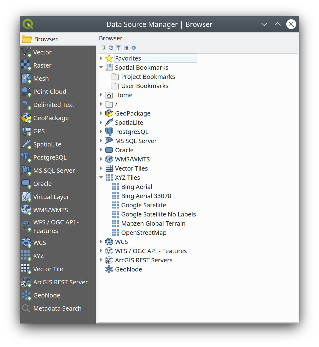
 DB tvarkyklė, kuris teikia galimybę analizuoti ir manipuliuoti prijungtas duomenų bazes. Daugiau informacijos apie DB tvarkyklės galimybes rasite skyriuje DB Manager Plugin.
 ) arba paspaudę Ctrl+2.
 Pridėti parinktus sluoksnius: jūs taipogi galite pridėti duomenis į žemėlapio drobę parinkdami sluoksnio kontekstiniame meniu Pridėti parinktą sluoksnį(ius);
 Atnaujinti naršyklės medį;
 Filtruoti naršyklę konkrečių duomenų paieškai. Įveskite paieškos žodį ar šabloną ir naršyklė filtruos medį, kad rodytų tik kelius į atitinkamas DB lenteles, failų pavadinimus ar aplankus – kiti duomenys ir aplankai nebus rodomi. Žiūrėkite naršyklės skydelio(2) pavyzdį Fig. 11.2. Lyginimą galima daryti atsižvelgiant į raidžių dydį arba ne. Jį taipogi galima nustatyti į:
 Sutraukti viską visą medį;
 Įjungti/išjungti savybių valdiklį: įjungus, naujas valdiklis pridedamas skydelio apačioje ir, kai galima, rodo parinkto elemento metaduomenis.
 GeoPackage
 SpatiaLite
 PostgreSQL
 SAP HANA
 MS SQL Serveris
 Oracle
 WMS/WMTS
 Vektorinės kaladėlės
 XYZ kaladėlės
 WCS
WCS WFS/OGC API-geoobjektai
 ArcGIS REST Serveris
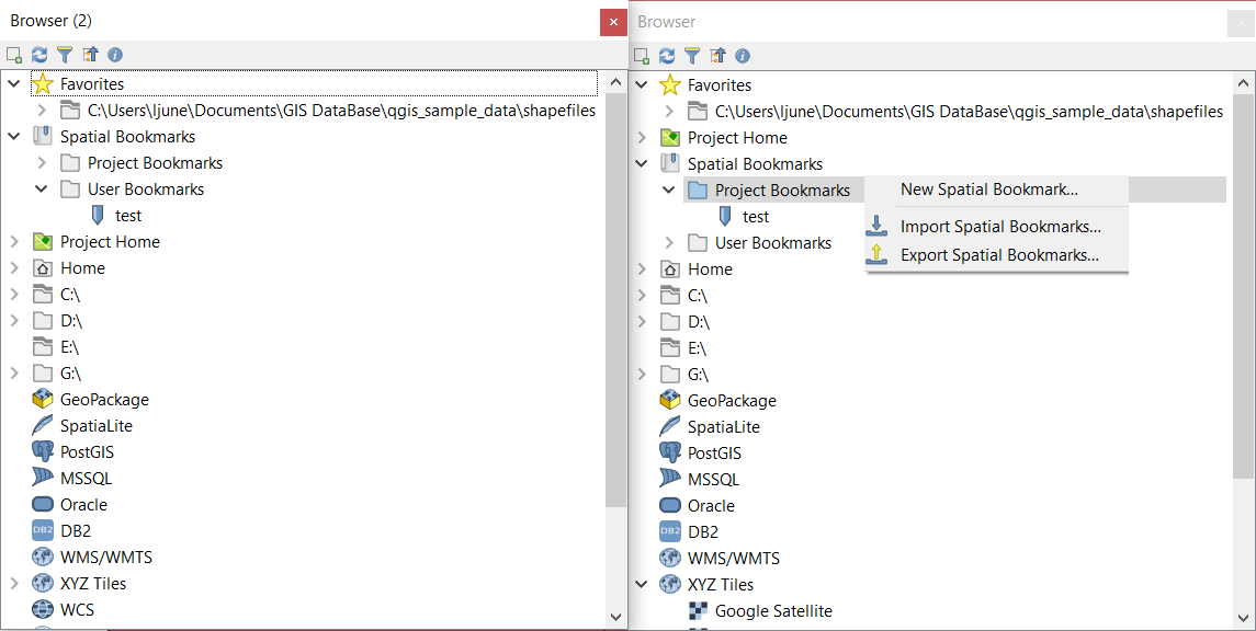
 Pridėti vektorinį sluoksnį arba spauskite įrankinės mygtuką
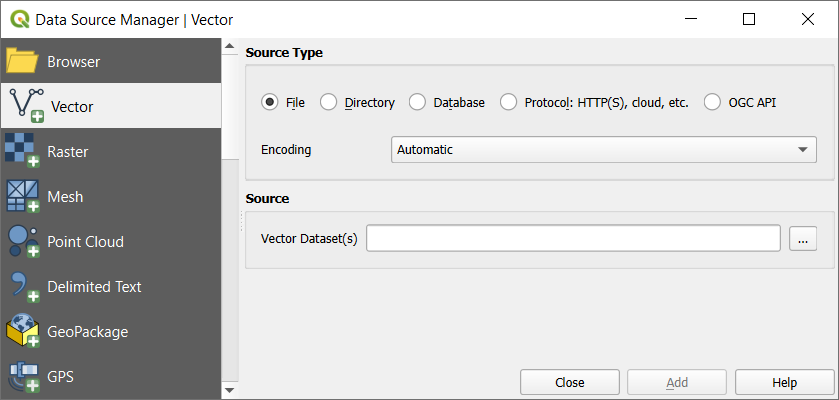
 Pridėti rastro sluoksnį arba spauskite įrankinės mygtuką
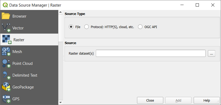
 Failas
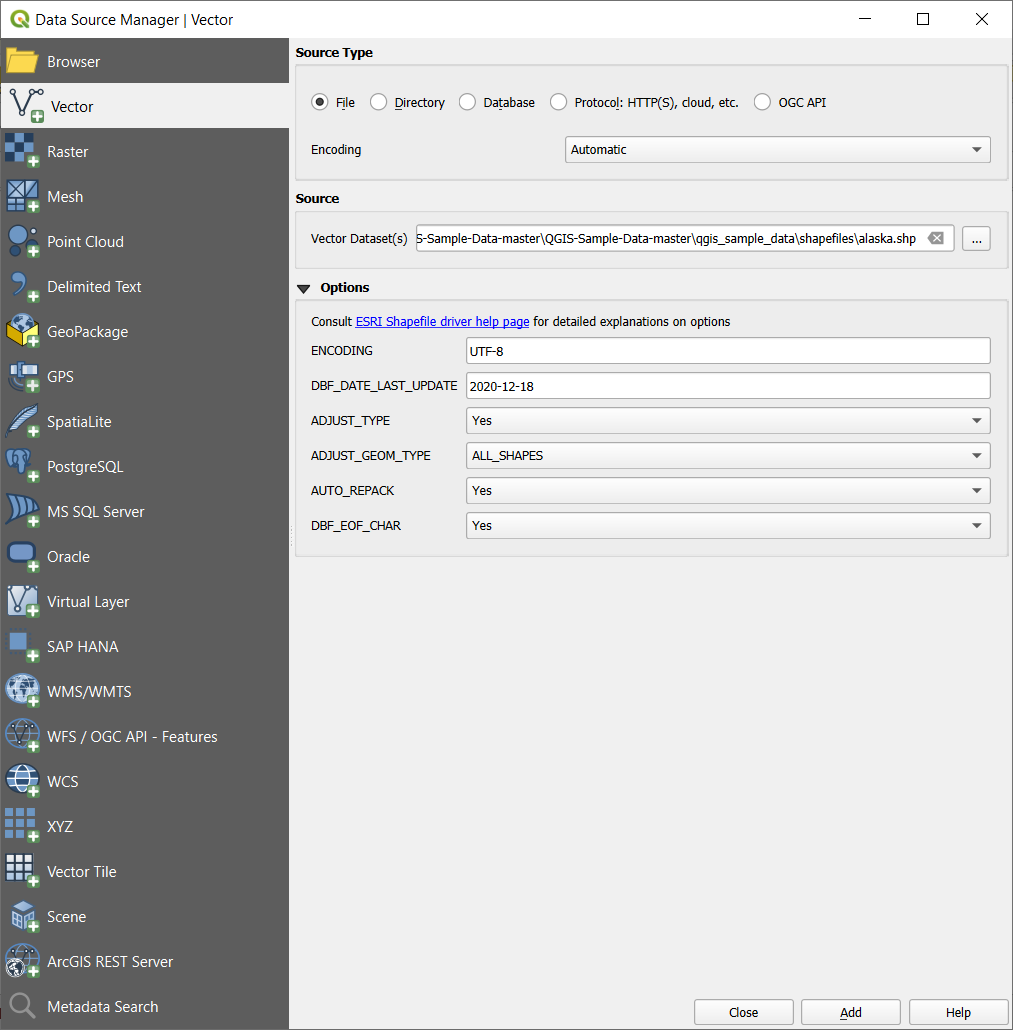
 Pridėti sluoksnius į grupę
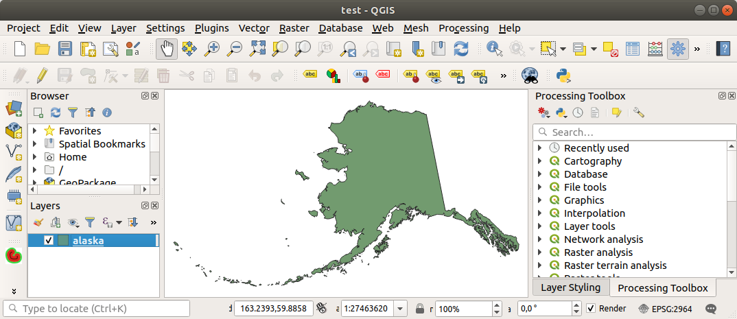
 Tinklelis
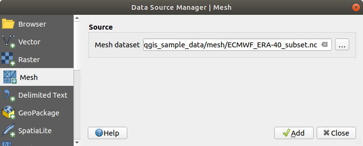
 Pridėti atskirtą teksto sluoksnį.
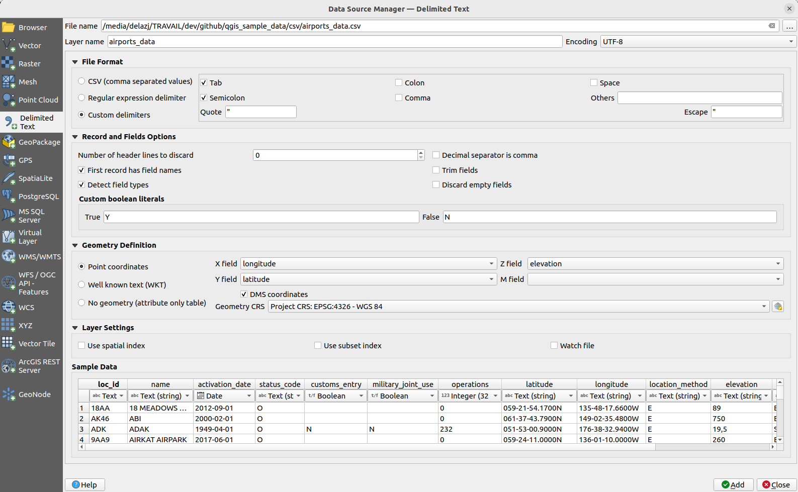
 Reguliarios išraiškos skirtukas ir įveskite tekstą į lauką Išraiška. Pavyzdžiui jei norite pakeisti skirtuką į tabuliacijos simbolį, naudokite
  Parinkti CRS.
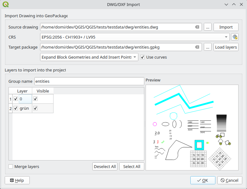
 Kai pirmą kartą įkeliate duomenis iš SpatiaLite duomenų bazės, pradėkite:
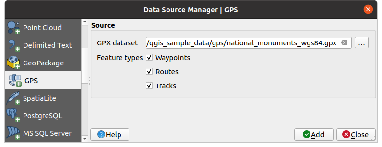
 ar paspaudus Ctrl+Shift+D
 ar paspaudus Ctrl+Shift+O
 ar paspaudus Ctrl+Shift+G
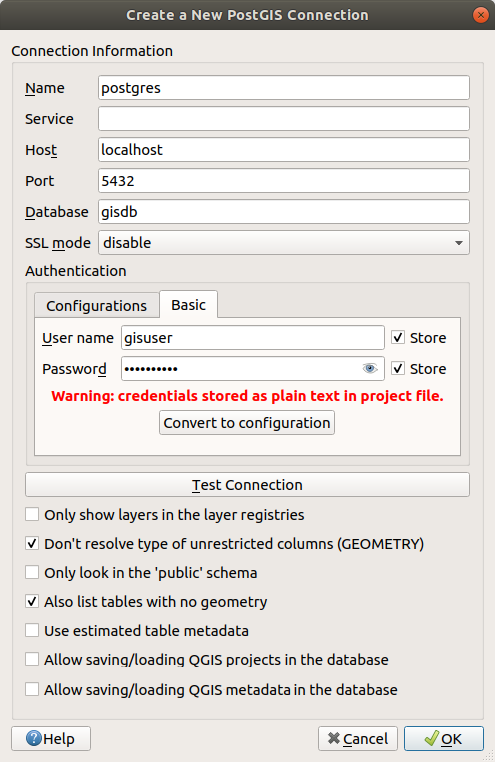
 . Pasirinkimai yra:
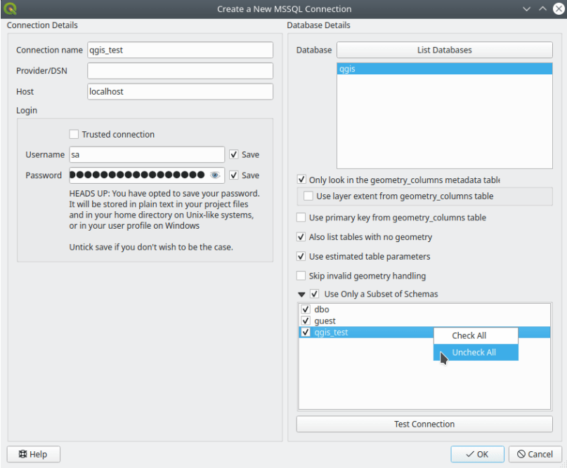
 : HANA ODBC tvarkyklės pavadinimas. Jis yra
 : arba pavadinimas, kuriuo buvo registruota SAP HANA ODBC tvarkyklė
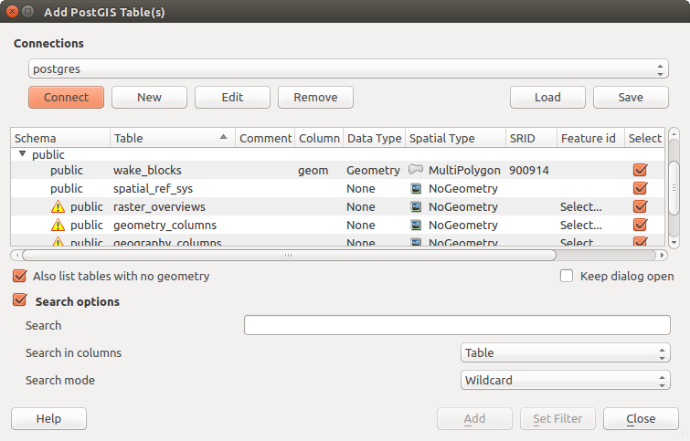
 Vektorinės kaladėlės, kurią rasite dialoge Duomenų šaltinių tvarkyklė ar įrašo Vektorinės kaladėlės kontekstiniame meniu Naršyklės skydelyje. Paslaugos gali būti arba Nauja bendra jungtis… arba Nauja ArcGIS vektorinių kaladėlių paslaugos jungtis….
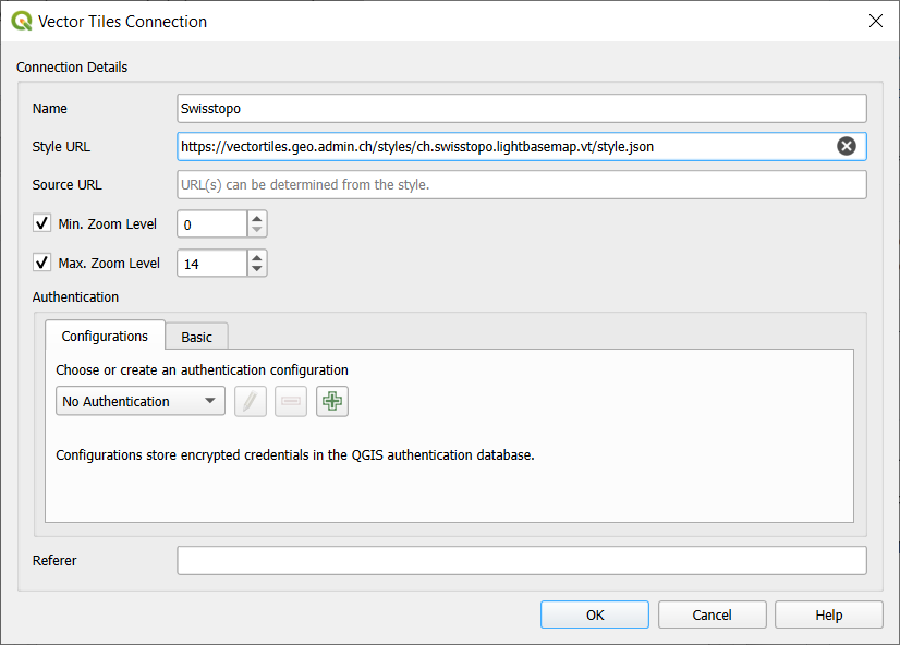
 XYZ, kurią rasite dialoge Duomenų šaltinių tvarkyklė arba XYZ kaladėlių įrašo kontekstiniame meniu Naršyklės skydelyje. Pagal nutylėjimą QGIS teikia kelias naudojimui paruoštas XYZ kaladėlių paslaugas:
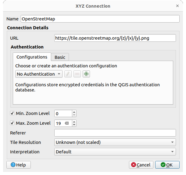
 ArcGIS REST Serveris, kurią rasite dialoge Duomenų šaltinių tvarkyklė arba ArcGIS REST Serverių įrašo kontekstiniame meniu Naršyklės skydelyje. Spauskite Naujas (atitinkamai Nauja jungtis) ir nurodykite:
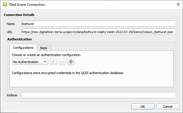
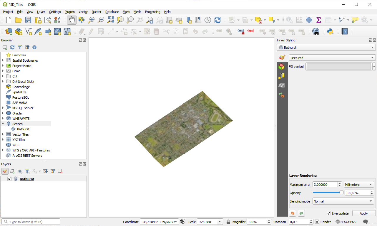
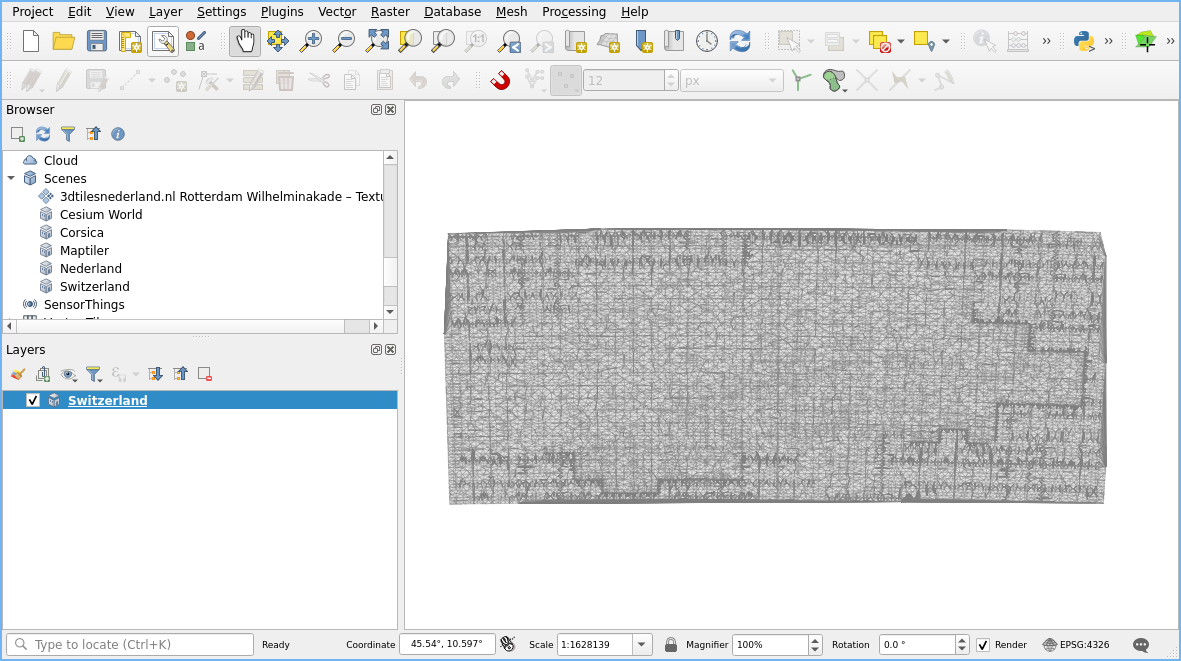
 Scena, kurią rasite dialoge Duomenų šaltinių tvarkyklė.
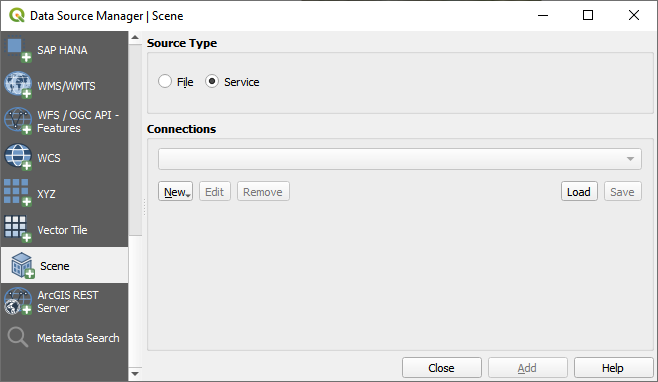
 Debesijos jungtį Naršyklės skydelyje spausdami dešinį mygtuką ant įrašo Debesija ir parinkdami Nauja jungtis. Jūs pamatysite galimų debesijos paslaugų iškrentantį sąrašą. Parinkite jums reikiamą paslaugą, prie kurios norite prisijungti, ir užpildykite reikiamus laukus: