Svarbu

Vertimas yra bendruomenės pastangos, prie kurių jūs galite prisijungti. Šis puslapis šiuo metu išverstas 61.33%.

11.3. Geo-koordinavimas

Geo-koordinatorius yra įrankis, skirtas nekoordinuotų rastro ar vektorinių sluoksnių pririšimui prie žinomų koordinačių sistemų naudojant žemės kontrolės taškus (GCP). Jis leidžia eksportuoti transformuotus rastrus (GeoTIFF) ir vektorius (shape failus, geopackages ir t.t.) ar įrašyti atitinkamus pasaulio failus (tik rastrams). Bazinis sluoksnio geo-koordinavimo būdas yra surasti jo taškus, kuriems jūs galite tiksliai nurodyti koordinates.

Savybės

Piktograma	Tikslas	Piktograma	Tikslas
	Atverti rastrą		Atverti vektorių
	Pradėti geo-koordinavimą
	Kurti GDAL skriptą		Įkelti GCP taškus
	Įrašyti GCP taškus kaip		Transformavimo nustatymai
	Pridėti GCP tašką		Trinti GCP tašką
	Perkelti GCP tašką		Pastumti
	Priartinti		Nutolinti
	Priartinti prie sluoksnio		Paskutinis mastelis
	Kitas mastelis		Susieti geo-koordinatorių su QGIS
	Susieti QGIS su geo-koordinatoriumi		Pilna histogramos apimtis
	Vietinė histogramos apimtis

Lentelė geo-koordinatorius: geo-koordinavimo įrankiai

11.3.1. Rastro sluoksnio geo-koordinavimas 

Nurodant X ir Y kordinates (DMS (dd mm ss.ss), DD (dd.dd) ar projektuotos koordinatės (mmmm.mm)), kurios atitinka piešinyje parinktą tašką, galima naudoti vieną iš dviejų būdų:

Kartais pačiame rastre yra kryžiukai su koordinatėmis „užrašytomis“ ant piešinio. Tokiu atveju jūs galite įvesti koordinates rankiniu būdu.
Galima naudoti jau geo-koordinuotus sluoksnius. Tai gali būti vektoriniai arba rastro duomenys, kuriuose yra tie patys objektai/geoobjektai, kaip ir piešinyje, kurį jūs norite geo-koordinuoti. Tokiu atveju galite įvesti koordinates paspausdami atskaitos duomenų rinkinį, įkeltą į QGIS žemėlapio drobę.

Įprastinė piešinio geo-koordinavimo procedūra yra parinkti kelis taškus rastre, nurodant jų koordinates, tada parenkant transformacijos tipą. Priklausomai nuo įvesties parametrų ir duomenų, Geo-koordinatorius paskaičiuos pasaulio failo parametrus. Kuo daugiau pateiksite koordinačių, tuo geresnis bus rezultatas.

Pirmas žingsnis yra paleisti QGIS ir spausti Sluoksnis ► Geo-koordinatorius, kurį jūs rasite QGIS meniu juostoje. Pasirodys geo-koordinatoriaus dialogas, kaip pavaizduota Fig. 11.34.

Šiam pavyzdžiui mes naudojame Šiaurės Dakotos SDGS topo lapą. Jį vėliau galima vizualizuoti kartu su duomenimis iš GRASS vietos spearfish60. Galite atsisiųsti topo lapą iš čia: https://grass.osgeo.org/sampledata/spearfish_toposheet.tar.gz.

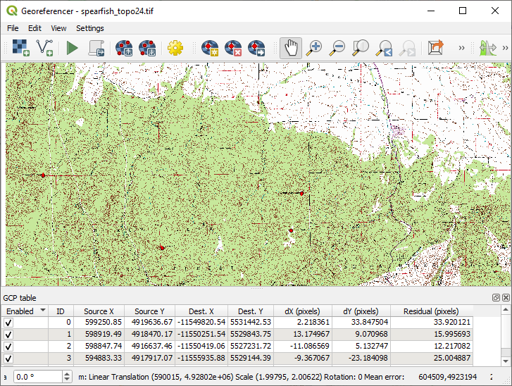
../../../_images/georef.png — Fig. 11.34 Geo-koordinavimo dialogas

11.3.1.1. Žemės kontrolinių taškų (GCP) įvedimas 

Norėdami pradėti geo-koordinuoti nepririštą rastrą, mes visų pirma turime jį įsikelti mygtuku . Rastras pasirodys pagrindiniame dialogo darbo plote. Įkėlus rastrą mes galime pradėti įvedinėti kontrolinius taškus.
Naudodami mygtuką ^{Pridėti GCP tašką}, pridėkite taškus į pagrindinį darbo plotą ir įveskite jų koordinates (žr. iliustraciją Fig. 11.35). Tam turite kelis būdus:
- Spauskite tašką rastro piešyje ir tada įveskite X ir Y koordinates rankiniu būdu, kartu su taško CRS.
- Spauskite tašką rastro piešinyje ir parinkite mygtuką ^{Iš žemėlapio drobės}, kad pridėtumėte X ir Y koordinates, naudodami jau geo-koordinuotą žemėlapį, kuris įkeltas QGIS žemėlapio drobėje. CRS bus nustatyta automatiškai.
- Įvesdami GCP iš pagrindinės žemėlapio drobės, galite pasirinkti paslėpti geo-koordinatoriaus langą, kol parenkate taškus pagrindinėje drobėje. Jei įjungta parinktis Automatiškai slėpti geo-koordinatoriaus langą, paspaudus Iš žemėlapio drobės, geo-koordinatoriaus langas bus paslėptas, kol žemėlapio drobėje nepridėsite taško. Dialogas Įveskite žemėlapio koordinates liks atvertas. Jei parinktis neįjungta, abu langai liks atidaryti parenkant taškus žemėlapio drobėje. Ši parinktis įsigalioja tik kai geo-koordinavimo langas nėra prisegtas pagrindinėje naudotojo sąsajoje.
Toliau pridėkite taškus. Turtėtumėte pridėti bent keturis taškus, kuo daugiau koordinačių galėsite pateikti, tuo geresnis bus rezultatas. Yra papildomi įrankiai darbo ploto priartinimui ar pastūmimui, kad galėtumėte rasti atitinkamus GCP taškus.

Patarimas

Kad išvengtumėte pastovaus persijunginėjimo tarp mygyukų ^Pastumti, ^{Pridėti GCP tašką} ir ^{Perkelti GCP tašką}, jūs galite naudoti klavišus judėjimui ir pelės ratuką patogiam geo-koordinavimo žemėlapio mastelio keitimui.
Kai pateiksite kelis taškus, galite naudoti mygtukus ^{Susieti QGIS su geo-koordinatoriumi} ir/ar ^{Susieti geo-koordinatorių su QGIS}, kad atitinkamai pakeistumėte pagrindinio QGIS lango vaizdą, kad jis rodytų geo-koordinatoriaus vaizdą arba atvirkščiai.
Su įrankiu jūs galite perkelti GCP tiek drobėje, tiek ir geo-koordinavimo lange, jei jums reikia juos patikslinti.

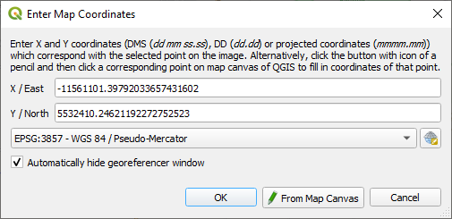
../../../_images/choose_points.png — Fig. 11.35 Pridėti taškus rastro piešinyje

Į žemėlapį pridėti taškai bus saugomi atskirame tekstiniame faile ([failovardas].points), paprastai kartu su rastro piešiniu. Tai leis mums vėliau iš naujo atidaryti geo-koordinatorių ir pridėti naujus taškus arba ištrinti esamus, kad pagerintumėme rezultatą. Taškų faile yra reikšmės iš: mapX, mapY, pixelX, pixelY. Jūs galite naudoti mygtukus ^{Įkelti GCP taškus} ir ^{Įrašyti GCP taškus kaip}, kad tvarkytumėte šiuos failus.

11.3.1.2. Defining the transformation settings 

After you have added your GCPs to the raster image, you need to define the transformation settings for the georeferencing process.

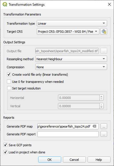
../../../_images/transformation_settings.png — Fig. 11.36 Defining the georeferencer transformation settings

Available Transformation algorithms 

A number of transformation algorithms are available, dependent on the type and quality of input data, the nature and amount of geometric distortion that you are willing to introduce to the final result, and the number of ground control points (GCPs).

Currently, the following Transformation types are available:

The Linear algorithm is used to create a world file and is different from the other algorithms, as it does not actually transform the raster pixels. It allows positioning (translating) the image and uniform scaling, but no rotation or other transformations. It is the most suitable if your image is a good quality raster map, in a known CRS, but is just missing georeferencing information. At least 2 GCPs are needed.
The Helmert transformation also allows rotation. It is particularly useful if your raster is a good quality local map or orthorectified aerial image, but not aligned with the grid bearing in your CRS. At least 2 GCPs are needed.
The Polynomial 1 algorithm allows a more general affine transformation, in particular also a uniform shear. Straight lines remain straight (i.e., collinear points stay collinear) and parallel lines remain parallel. This is particularly useful for georeferencing data cartograms, which may have been plotted (or data collected) with different ground pixel sizes in different directions. At least 3 GCP’s are required.
The Polynomial algorithms 2-3 use more general 2nd or 3rd degree polynomials instead of just affine transformation. This allows them to account for curvature or other systematic warping of the image, for instance photographed maps with curving edges. At least 6 (respectively 10) GCP’s are required. Angles and local scale are not preserved or treated uniformly across the image. In particular, straight lines may become curved, and there may be significant distortion introduced at the edges or far from any GCPs arising from extrapolating the data-fitted polynomials too far.
The Projective algorithm generalizes Polynomial 1 in a different way, allowing transformations representing a central projection between 2 non-parallel planes, the image and the map canvas. Straight lines stay straight, but parallelism is not preserved and scale across the image varies consistently with the change in perspective. This transformation type is most useful for georeferencing angled photographs (rather than flat scans) of good quality maps, or oblique aerial images. A minimum of 4 GCPs is required.
Finally, the Thin Plate Spline (TPS) algorithm „rubber sheets“ the raster using multiple local polynomials to match the GCPs specified, with overall surface curvature minimized. Areas away from GCPs will be moved around in the output to accommodate the GCP matching, but will otherwise be minimally locally deformed. TPS is most useful for georeferencing damaged, deformed, or otherwise slightly inaccurate maps, or poorly orthorectified aerials. It is also useful for approximately georeferencing and implicitly reprojecting maps with unknown projection type or parameters, but where a regular grid or dense set of ad-hoc GCPs can be matched with a reference map layer. It technically requires a minimum of 10 GCPs, but usually more to be successful.

In all of the algorithms except TPS, if more than the minimum GCPs are specified, parameters will be fitted so that the overall residual error is minimized. This is helpful to minimize the impact of registration errors, i.e. slight imprecisions in pointer clicks or typed coordinates, or other small local image deformations. Absent other GCPs to compensate, such errors or deformations could translate into significant distortions, especially near the edges of the georeferenced image. However, if more than the minimum GCPs are specified, they will match only approximately in the output. In contrast, TPS will precisely match all specified GCPs, but may introduce significant deformations between nearby GCPs with registration errors.

Define the Resampling method 

The type of resampling you choose will likely depend on your input data and the ultimate objective of the exercise. If you don’t want to change statistics of the raster (other than as implied by nonuniform geometric scaling if using other than the Linear, Helmert, or Polynomial 1 transformations), you might want to choose ‚Nearest neighbour‘. In contrast, ‚cubic resampling‘, for instance, will usually generate a visually smoother result.

It is possible to choose between five different resampling methods:

Nearest neighbour
Bilinear (2x2 kernel)
Cubic (4x4 kernel)
Cubic B-Spline (4x4 kernel)
Lanczos (6x6 kernel)

Define the transformation settings 

There are several options that need to be defined for the georeferenced output raster.

The Create world file checkbox is only available if you decide to use the linear transformation type, because this means that the raster image actually won’t be transformed. In this case, the Output raster field is not activated, because only a new world file will be created.
For all other transformation types, you have to define an Output raster. As default, a new file ([filename]_modified) will be created in the same folder together with the original raster image.
As a next step, you have to define the Target CRS (Coordinate Reference System) for the georeferenced raster (see Darbas su projekcijomis).
If you like, you can generate a pdf map and also a pdf report. The report includes information about the used transformation parameters, an image of the residuals and a list with all GCPs and their RMS errors.
Furthermore, you can activate the Set Target Resolution checkbox and define the pixel resolution of the output raster. Default horizontal and vertical resolution is 1.
The Use 0 for transparency when needed can be activated, if pixels with the value 0 shall be visualized transparent. In our example toposheet, all white areas would be transparent.
The Save GCP Points will store GCP Points in a file next to the output raster.
Finally, Load in project when done loads the output raster automatically into the QGIS map canvas when the transformation is done.

11.3.1.3. Running the transformation 

After all GCPs have been collected and all transformation settings are defined, just press the ^{Start georeferencing} button to create the new georeferenced raster.

11.3.2. Georeferencing vector layer 

Georeferencing vector layers works similarly to raster georeferencing, but instead of matching image pixels, you match vector geometries (points, lines, or polygons) to known spatial references.

The standard procedure starts the same as for raster georeferencing: open QGIS and add a layer to the map canvas to use as a reference. This can be a georeferenced raster or vector layer, or a WMS layer.

Open the Georeferencer dialog from Layer ► Georeferencer.

Start georeferencing by following these steps (in this example, we use an unreferenced alaska.shp):

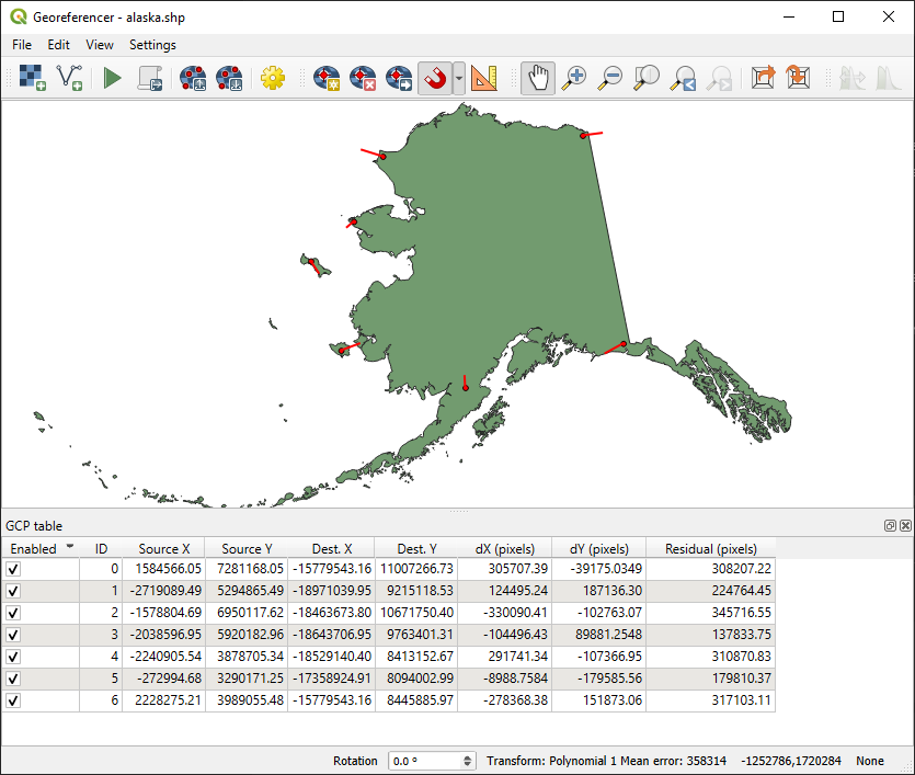
../../../_images/vector_georeferencer_dialog.png — Fig. 11.37 Vector Georeferencer Dialog

Load the unreferenced vector layer using the button. The vector layer will appear in the main working area of the dialog.
Use the ^{Add GCP Point} button to add a point to the working area. Enter its coordinates manually and set the CRS, or click the ^{From map canvas} button to pick the coordinates from a georeferenced layer in the main QGIS map canvas. In that case, the CRS will be set automatically.
Define the transformation settings:
- Select the Transformation type. The transformation algorithms are the same as those for raster georeferencing. See Defining the transformation settings for more details.
- Define the Target CRS (Coordinate Reference System) for the georeferenced vector (see Darbas su projekcijomis).
- Set the output file format and path (e.g., GeoPackage, Shapefile). By default, a new file with suffix _modified will be created in the same folder as the original vector file.
- Optionally, enable Generate PDF map and Generate PDF report. The report includes transformation parameters, GCP residuals, and a summary of RMS errors.
- Enable Save GCP Points to store GCPs in a file alongside the output vector layer.
- Enable Load in project when done to add the result directly to the map canvas.
Click ^{Start georeferencing} to run the transformation and generate the georeferenced vector layer.

11.3.3. Show and adapt layer properties 

Clicking on the Source properties option in the Settings menu opens the Raster Layer properties or Vector Layer properties depending on the type of layer you are georeferencing.

11.3.4. Configure the georeferencer 

You can customize the behavior of the georeferencer in Settings ► Configure Georeferencer (or use keyboard shortcut Ctrl+P).

Under Point Tip you can use the checkboxes to toggle displaying GCP IDs and X/Y coordinates in both the Georeferencer window and the main map canvas.
Residual Units controls whether residual units are given in pixels or map units
PDF Report allows you to set margin size in mm for the report export
PDF Map allows you to choose a paper size for the map export
Finally, you can activate to Show Georeferencer window docked. This will dock the Georeferencer window in the main QGIS window rather than showing it as a separate window that can be minimized.