Important
La traduction est le fruit d’un effort communautaire auquel vous pouvez vous joindre. Cette page est actuellement traduite à 58.39%.
11.3. Géoréférencer
The  Georeferencer is a tool for aligning unreferenced raster or vector layers
to known coordinate systems using Ground Control Points (GCPs).
It supports exporting transformed rasters (GeoTIFF) and vectors (shapefiles, geopackages, etc.)
or writing accompanying world files (for raster only). The basic
approach to georeferencing a layer is to locate points on it for which
you can accurately determine coordinates.
Georeferencer is a tool for aligning unreferenced raster or vector layers
to known coordinate systems using Ground Control Points (GCPs).
It supports exporting transformed rasters (GeoTIFF) and vectors (shapefiles, geopackages, etc.)
or writing accompanying world files (for raster only). The basic
approach to georeferencing a layer is to locate points on it for which
you can accurately determine coordinates.
Fonctionnalités
Icône |
Fonction |
Icône |
Fonction |
|---|---|---|---|
|
Ouvrir un raster |
|
Ouvrir un vecteur |
|
Commencer le géoréférencement |
|
Générer le script GDAL |
|
Charger les points de contrôle |
|
Sauvegarder les points de contrôle |
|
Paramètres de transformation |
||
Ajouter les points de contrôle |
Add GCP Point |
Supprimer les points de contrôle |
Delete GCP Point |
Déplacer les points de contrôle |
Déplacer un point GCP |
|
Snapping Type |
|
Show Advanced Digitizing Dock |
|
Se déplacer |
|
Zoom + |
|
Zoom - |
|
Zoom sur la couche |
|
Zoom précédent |
|
Zoom suivant |
|
Lier le géoréférenceur à QGIS |
|
Lier QGIS au géoréférenceur |
|
Histogramme complet |
|
Histogramme de l’emprise locale |


11.3.1. Georeferencing raster layer
Pour déterminer des coordonnées X et Y (notées en DMS (dd mm ss.ss), DD (dd.dd) ou en coordonnées projetées (mmmm.mm)) qui correspondent au point sélectionné sur l’image, deux procédures peuvent être suivies :
Par le raster lui-même : quelquefois les coordonnées sont littéralement écrites (p. ex., les graticules). Dans ce cas, vous pouvez les saisir manuellement.
Par des données déjà géoréférencées. Il peut d’agir de données vecteur ou raster où figurent les mêmes objets/entités que sur le raster que vous désirez géoréférencer et dans le même système de projection. Dans ce cas, vous pouvez renseigner les coordonnées en cliquant sur les données de référence chargées dans la carte principale de QGIS.
La procédure standard pour le géoréférencement d’une image implique la sélection de plusieurs points sur l’image, en spécifiant leurs coordonnées et en choisissant la transformation appropriée. En se basant sur les paramètres entrés et les données, le Géoréférenceur calculera les paramètres du fichier « world ». Plus il y a de coordonnées fournies, meilleur sera le résultat.
La première étape consiste à lancer QGIS et à cliquer sur , qui apparaît dans la barre de menu de QGIS. Le dialogue géoréférencer apparaît comme indiqué dans Fig. 11.38.
En guise d’exemple, nous allons utiliser une carte topographique du Dakota du Sud publiée par le SDGS. Elle pourra par la suite être affichée avec les données du secteur GRASS spearfish60. Cette carte topographique peut être téléchargée à l’adresse suivante : https://grass.osgeo.org/sampledata/spearfish_toposheet.tar.gz.
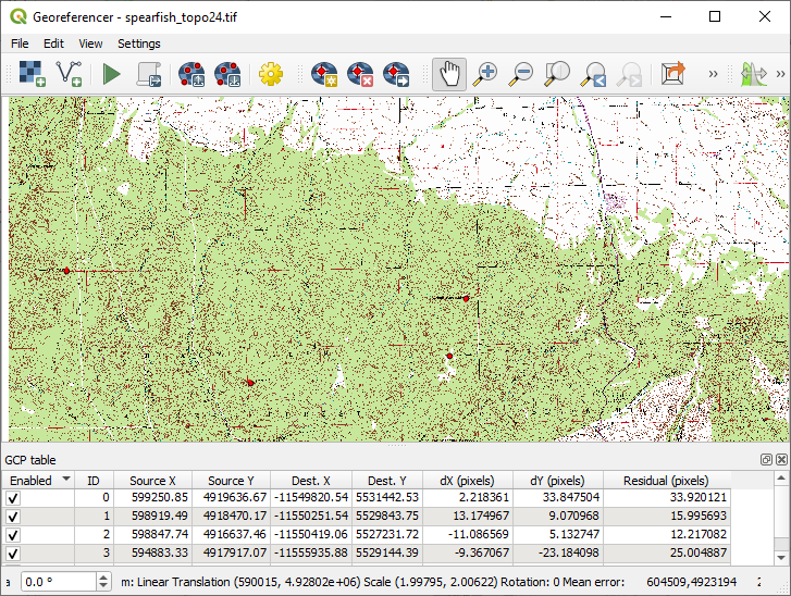
Fig. 11.38 Fenêtre de Géoréférencement
11.3.1.1. Saisir des points de contrôle (GCP)
Pour commencer le géoréférencement d’un raster, nous devons le charger via le bouton
 . Le raster apparaît alors dans la surface principale de travail de la fenêtre. Une fois qu’il est chargé, nous pouvons commencer à entrer des points de contrôles.
Using the
 Add GCP Point button, add points to the
main working area and enter their coordinates (see Figure Fig. 11.39).
For this procedure you have the following options:
Add GCP Point button, add points to the
main working area and enter their coordinates (see Figure Fig. 11.39).
For this procedure you have the following options:Click on a point in the raster image and enter the X and Y coordinates manually, along with the CRS of the point.
Click on a point in the raster image and choose the
 From map canvas button to add the X and Y coordinates with the help of a
georeferenced map already loaded in the QGIS map canvas. The CRS will be set
automatically.
From map canvas button to add the X and Y coordinates with the help of a
georeferenced map already loaded in the QGIS map canvas. The CRS will be set
automatically.When entering GCPs from the main map canvas, you have the option to hide the georeferencer window while selecting points from the main canvas. If the
 Automatically hide georeferencer window
checkbox is ticked, after clicking From Map Canvas,
the main georeferencer window will be hidden until a point is added on the
map canvas.
The Enter Map Coordinates dialog will remain open.
If the box is unchecked, both windows will remain open while selecting a
point on the map canvas.
This option only takes effect when the georeferencer window is not docked
in the main interface.
Automatically hide georeferencer window
checkbox is ticked, after clicking From Map Canvas,
the main georeferencer window will be hidden until a point is added on the
map canvas.
The Enter Map Coordinates dialog will remain open.
If the box is unchecked, both windows will remain open while selecting a
point on the map canvas.
This option only takes effect when the georeferencer window is not docked
in the main interface.
Continuez d’entrer des points. Vous devez en avoir au moins quatre et plus vous en ajoutez, meilleur sera le résultat. Des outils additionnels permettent de zoomer et de se déplacer dans l’espace de travail pour localiser les points de contrôle pertinents.
Astuce
To avoid constant switching between
 Pan, Add GCP point
and
Pan, Add GCP point
and  Move GCP point buttons,
you may use the keyboard arrow keys for moving and the mouse wheel for scaling the georeferenced map conveniently.
Move GCP point buttons,
you may use the keyboard arrow keys for moving and the mouse wheel for scaling the georeferenced map conveniently.After you provide a few points, you can use the
 Link QGIS to Georeferencer
and/or
Link QGIS to Georeferencer
and/or  Link Georeferencer to QGIS buttons that will adjust, respectively,
the map extent of the main QGIS window to the present view in Georeferencer and/or vice versa.
Link Georeferencer to QGIS buttons that will adjust, respectively,
the map extent of the main QGIS window to the present view in Georeferencer and/or vice versa.Si nécessaire, vous pouvez déplacer les points de contrôle à la fois dans le canevas et la fenêtre du géoréférenceur à l’aide de l’outil
.
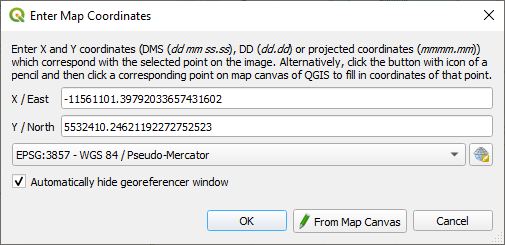
Fig. 11.39 Ajout de points de contrôle à l’image raster
Les points qui sont ajoutés sur la carte sont enregistrés dans un fichier texte distinct ([nomdufichier].points) qui est stocké avec le fichier image. Il permet de rouvrir le Géoréférenceur à une date ultérieure et de rajouter de nouveaux points ou d’effacer ceux existants pour améliorer le résultat sans devoir tout refaire. Le fichier de points contient les valeurs suivantes : mapX, mapY, pixelX, pixelY. Vous pouvez utiliser les boutons  Charger des points de contrôle et
  Sauvegarder des points de contrôle pour gérer ces fichiers.
11.3.1.2. Configurer la transformation
Après avoir ajouté vos points de contrôle, vous devez sélectionner la méthode de transformation qui sera utilisée pour le géoréférencement.
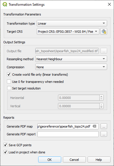
Fig. 11.40 Définir les paramètres de transformation pour le géoréférencement
Algorithmes de transformation disponibles
A number of transformation algorithms are available, dependent on the type and quality of input data, the nature and amount of geometric distortion that you are willing to introduce to the final result, and the number of ground control points (GCPs).
Actuellement les types de transformation suivants sont disponibles :
The Linear algorithm is used to create a world file and is different from the other algorithms, as it does not actually transform the raster pixels. It allows positioning (translating) the image and uniform scaling, but no rotation or other transformations. It is the most suitable if your image is a good quality raster map, in a known CRS, but is just missing georeferencing information. At least 2 GCPs are needed.
The Helmert transformation also allows rotation. It is particularly useful if your raster is a good quality local map or orthorectified aerial image, but not aligned with the grid bearing in your CRS. At least 2 GCPs are needed.
The Polynomial 1 algorithm allows a more general affine transformation, in particular also a uniform shear. Straight lines remain straight (i.e., collinear points stay collinear) and parallel lines remain parallel. This is particularly useful for georeferencing data cartograms, which may have been plotted (or data collected) with different ground pixel sizes in different directions. At least 3 GCP’s are required.
The Polynomial algorithms 2-3 use more general 2nd or 3rd degree polynomials instead of just affine transformation. This allows them to account for curvature or other systematic warping of the image, for instance photographed maps with curving edges. At least 6 (respectively 10) GCP’s are required. Angles and local scale are not preserved or treated uniformly across the image. In particular, straight lines may become curved, and there may be significant distortion introduced at the edges or far from any GCPs arising from extrapolating the data-fitted polynomials too far.
The Projective algorithm generalizes Polynomial 1 in a different way, allowing transformations representing a central projection between 2 non-parallel planes, the image and the map canvas. Straight lines stay straight, but parallelism is not preserved and scale across the image varies consistently with the change in perspective. This transformation type is most useful for georeferencing angled photographs (rather than flat scans) of good quality maps, or oblique aerial images. A minimum of 4 GCPs is required.
Finally, the Thin Plate Spline (TPS) algorithm « rubber sheets » the raster using multiple local polynomials to match the GCPs specified, with overall surface curvature minimized. Areas away from GCPs will be moved around in the output to accommodate the GCP matching, but will otherwise be minimally locally deformed. TPS is most useful for georeferencing damaged, deformed, or otherwise slightly inaccurate maps, or poorly orthorectified aerials. It is also useful for approximately georeferencing and implicitly reprojecting maps with unknown projection type or parameters, but where a regular grid or dense set of ad-hoc GCPs can be matched with a reference map layer. It technically requires a minimum of 10 GCPs, but usually more to be successful.
In all of the algorithms except TPS, if more than the minimum GCPs are specified, parameters will be fitted so that the overall residual error is minimized. This is helpful to minimize the impact of registration errors, i.e. slight imprecisions in pointer clicks or typed coordinates, or other small local image deformations. Absent other GCPs to compensate, such errors or deformations could translate into significant distortions, especially near the edges of the georeferenced image. However, if more than the minimum GCPs are specified, they will match only approximately in the output. In contrast, TPS will precisely match all specified GCPs, but may introduce significant deformations between nearby GCPs with registration errors.
Définir la méthode de rééchantillonage
The type of resampling you choose will likely depend on your input data and the ultimate objective of the exercise. If you don’t want to change statistics of the raster (other than as implied by nonuniform geometric scaling if using other than the Linear, Helmert, or Polynomial 1 transformations), you might want to choose “Nearest neighbour”. In contrast, “cubic resampling”, for instance, will usually generate a visually smoother result.
Il est possible de choisir entre 5 méthodes de ré-échantillonnage :
Plus proche voisin
Bilinear (2x2 kernel)
Cubic (4x4 kernel)
Cubic B-Spline (4x4 kernel)
Lanczos (6x6 kernel)
Define the Raster creation options
When exporting a raster, Raster creation options allows you to define
additional options that control how the output file is structured and compressed.
See more at Raster driver options.
Astuce
Select an empty entry if you want to create your own custom combination of parameters.
Définir les paramètres de transformation
Plusieurs paramètres doivent être renseignés afin de créer un raster géoréférencé.
La case
Créer un fichier de coordonnées est uniquement disponible lorsque la méthode de transformation linéaire est choisie, et ce, parce que votre image ne sera alors pas transformée en sortie. Dans ce cas précis, le champ raster de sortie ne sera pas activé, car seul le fichier de coordonnées sera créé.Pour tous les autres types de transformations, vous pouvez saisir un Raster de sortie. Par défaut, le nouveau fichier s’intitulera ([nomdefichier]_georef) et sera enregistré dans le même répertoire que le raster original.
As a next step, you have to define the Target CRS (Coordinate Reference System) for the georeferenced raster (see Utiliser les projections).
Si vous le désirez, vous pouvez demander à générer une carte PDF ou générer un rapport PDF qui inclut tous les paramètres définis ainsi qu’une image avec tous les résidus et une liste des points de contrôles et leurs erreurs RMS.
Vous pouvez cocher la case
Définir la résolution de la cible et préciser la résolution de pixel du raster généré. La résolution horizontale et verticale par défaut est de 1.Lorsque la case
Employer 0 pour la transparence si nécessaire est cochée, cela indique que la valeur 0 sera transparente lors de la visualisation. Dans notre exemple, toutes les zones blanches seront transparentes.The
Save GCP Points will store GCP Points in a file next
to the output raster.Finally,
Load in project when done loads the output raster
automatically into the QGIS map canvas when the transformation is done.
11.3.1.3. Lancer la transformation
Lorsque tous les points de contrôle ont été posés et les paramètres de transformation saisis, appuyez sur le bouton  Commencer le géoréférencement pour créer le raster final.
11.3.2. Georeferencing vector layer
Georeferencing vector layers works similarly to raster georeferencing, but instead of matching image pixels, you match vector geometries (points, lines, or polygons) to known spatial references.
The standard procedure starts the same as for raster georeferencing: open QGIS and add a layer to the map canvas to use as a reference. This can be a georeferenced raster or vector layer, or a WMS layer.
Open the Georeferencer dialog from .
Start georeferencing by following these steps (in this example, we use an unreferenced alaska.shp):
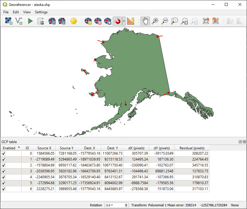
Fig. 11.41 Fenêtre de géoréférencement d’une couche vecteur
Load the unreferenced vector layer using the
 button.
The vector layer will appear in the main working area of the dialog.
button.
The vector layer will appear in the main working area of the dialog.Activate snapping by clicking the
 button and selecting the desired snapping type(s).
This enables snapping to the reference layer when placing GCPs.
button and selecting the desired snapping type(s).
This enables snapping to the reference layer when placing GCPs.You can also use the
 Advanced Digitizing dock to ensure high-precision
point selection. For more information, refer to the
Advanced Digitizing section.
Advanced Digitizing dock to ensure high-precision
point selection. For more information, refer to the
Advanced Digitizing section.Use the
Add GCP Point button to add a point to the working area.
Enter its coordinates manually and set the CRS, or click the From map canvas button
to pick the coordinates from a georeferenced layer in the main QGIS map canvas.
In that case, the CRS will be set automatically.Define the transformation settings:
Select the Transformation type. The transformation algorithms are the same as those for raster georeferencing. See Configurer la transformation for more details.
Define the Target CRS (Coordinate Reference System) for the georeferenced vector (see Utiliser les projections).
Set the output file format and path (e.g., GeoPackage, Shapefile). By default, a new file with suffix
_modifiedwill be created in the same folder as the original vector file.Optionally, enable Generate PDF map and Generate PDF report. The report includes transformation parameters, GCP residuals, and a summary of RMS errors.
Enable
Save GCP Points to store GCPs in a file alongside the output vector layer.Enable
Load in project when done to add the result directly to the map canvas.
Click
Start georeferencing to run the transformation and generate the georeferenced vector layer.
11.3.3. Afficher et modifier les propriétés raster
Clicking on the Source properties option in the Settings menu opens the Raster Layer properties or Vector Layer properties depending on the type of layer you are georeferencing.
11.3.4. Configurer le géoreferenceur
You can customize the behavior of the georeferencer in (or use keyboard shortcut Ctrl+P).
Under Point Tip you can use the checkboxes to toggle displaying GCP IDs and X/Y coordinates in both the Georeferencer window and the main map canvas.
Residual Units controls whether residual units are given in pixels or map units
PDF Report allows you to set margin size in mm for the report export
PDF Map allows you to choose a paper size for the map export
Finally, you can activate to
Show Georeferencer window
docked.
This will dock the Georeferencer window in the main QGIS window rather than
showing it as a separate window that can be minimized.