17.17. Iniciando com o modelador gráfico

Nota

Nesta lição usaremos o modelador gráfico, um poderoso componente que podemos usar para definir um fluxo de trabalho e executar uma cadeia de algoritmos.

Uma sessão normal com as ferramentas de processamento incluem mais do que rodar um único algoritmo. Normalmente, vários deles são executados para se obter um resultado, e as saídas de alguns destes códigos são usados como entrada para outros.

Usando o modelador gráfico, o fluxo de trabalho pode ser colocado em um modelo, que rodará todos os algoritmos necessários em uma única execução, simplificando, assim, todo o processo e o automatizando.

To start this lesson, we are going to calculate a parameter named Topographic Wetness Index. The algorithm that computes it is called Topographic wetness index (twi).

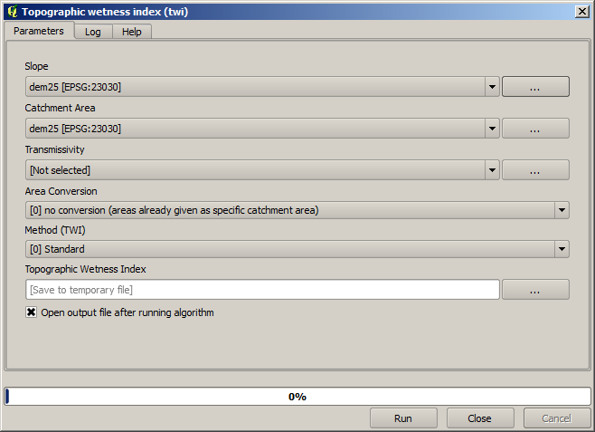
Como você pode ver, existem duas entradas obrigatórias: Slope e Área de Captação. Há também uma entrada opcional, porém você não poderá usá-la, então ignore-a.

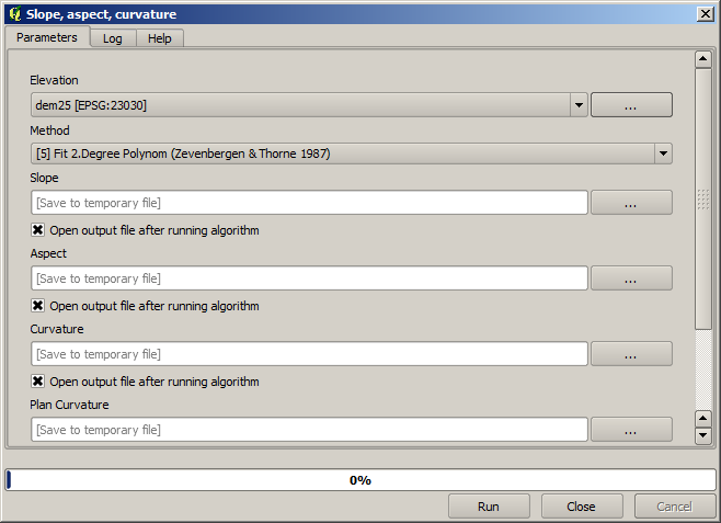
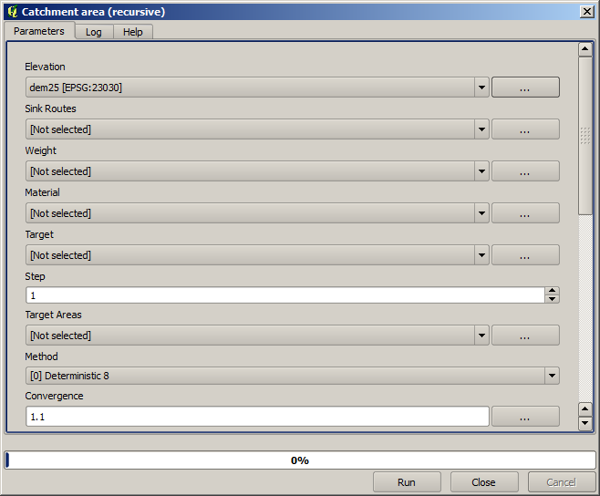
Los datos para esta lección contienen sólo un MDT, así que no tenemos ninguna de las entradas requeridas. Sin embargo, conocemos cómo calcular ambos a partir de ese MDT, como ya hemos visto los algoritmos para calcular pendiente y zona de captación. Así que lo primero que podemos calcular son esas capas y entonces utilizarlos para el algoritmo TWI.

Aquí esta el diálogo de parámetros que debería utilizar para calcular las capas intermedias.

Nota

A declividade será calculada em radiano, não em graus.

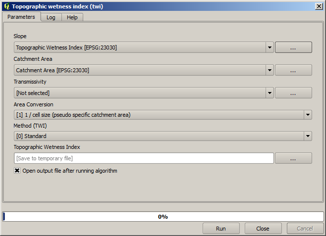
Y esto es cómo tener que establecer el diálogo de parámetros del algoritmo TWI.

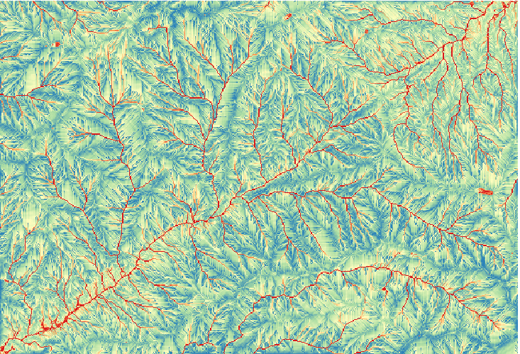
This is the result that you will obtain (the default singleband pseudocolor inverted palette has been used for rendering). You can use the twi.qml style provided.

What we will try to do now is to create an algorithm that calculates the TWI from a DEM in just one single step. That will save us work in case we later have to compute a TWI layer from another DEM, since we will need just one single step to do it instead of the three above. All the processes that we need are found in the toolbox, so what we have to do is to define the workflow to wrap them. This is where the graphical modeler comes in.

1. Abra el modelador seleccionando su entrada de menú en el menú procesamiento.

   

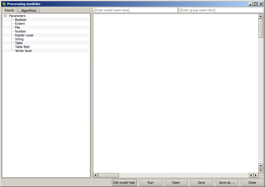
   Two things are needed to create a model: setting the inputs that it will need, and defining the algorithm that it contains. Both of them are done by adding elements from the two tabs in the left-hand side of the modeler window: Inputs and Algorithms.

2. Vamos a empezar con las entradas. En este caso no tenemos mucho que añadir. Sólo necesitamos una capa ráster con el MDT y que serán nuestros únicos datos de entrada.

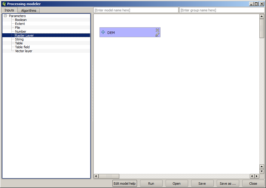
3. Double click on the Raster layer input and you will see the following dialog.

   

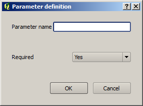
4. Aqui teremos que definir a entrada que queremos:

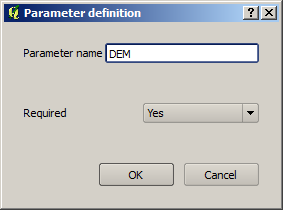
   1. Since we expect this raster layer to be a DEM, we will call it DEM. That’s the name that the user of the model will see when running it.

   2. Como precisamos que essa camada funcione, vamos defini-la como uma camada obrigatória.

   Aquí esta cómo el diálogo debería ser configurado.

   

5. Click on OK and the input will appear in the modeler canvas.

   

6. Now let’s move to the Algorithms tab.

7. The first algorithm we have to run is the Slope, aspect, curvature algorithm. Locate it in the algorithm list, double-click on it and you will see the dialog shown below.

   

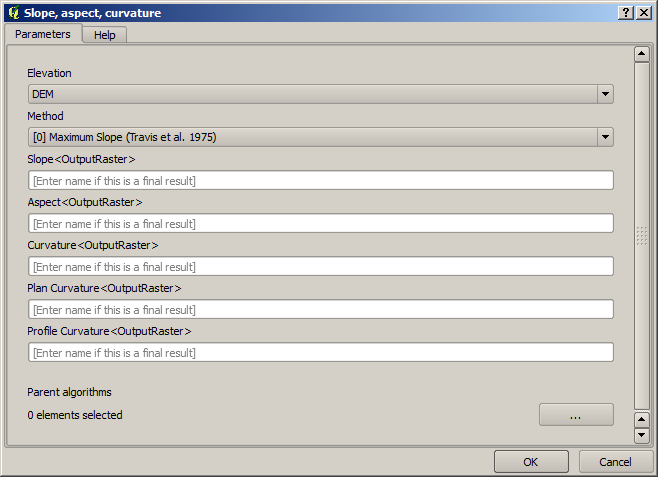
   This dialog is very similar to the one that you can find when running the algorithm from the toolbox, but the element that you can use as parameter values are not taken from the current QGIS project, but from the model itself. That means that, in this case, we will not have all the raster layers of our project available for the Elevation field, but just the ones defined in our model. Since we have added just one single raster input named DEM, that will be the only raster layer that we will see in the list corresponding to the Elevation parameter.

   Output generated by an algorithm are handled a bit differently when the algorithm is used as a part of a model. Instead of selecting the filepath where you want to save each output, you just have to specify if that output is an intermediate layer (and you do not want it to be preserved after the model has been executed), or it is a final one. In this case, all layers produced by this algorithm are intermediate. We will only use one of them (the slope layer), but we do not want to keep it, since we just need it to calculate the TWI layer, which is the final result that we want to obtain.

   Cuando las capas no son un resultado final, sólo debe dejar el campo correspondiente. De lo contrario, se tiene que introducir un nombre que se utilizará para identificar la capa en el diálogo de parámetros que se mostrará cuando ejecute el modelo posterior.

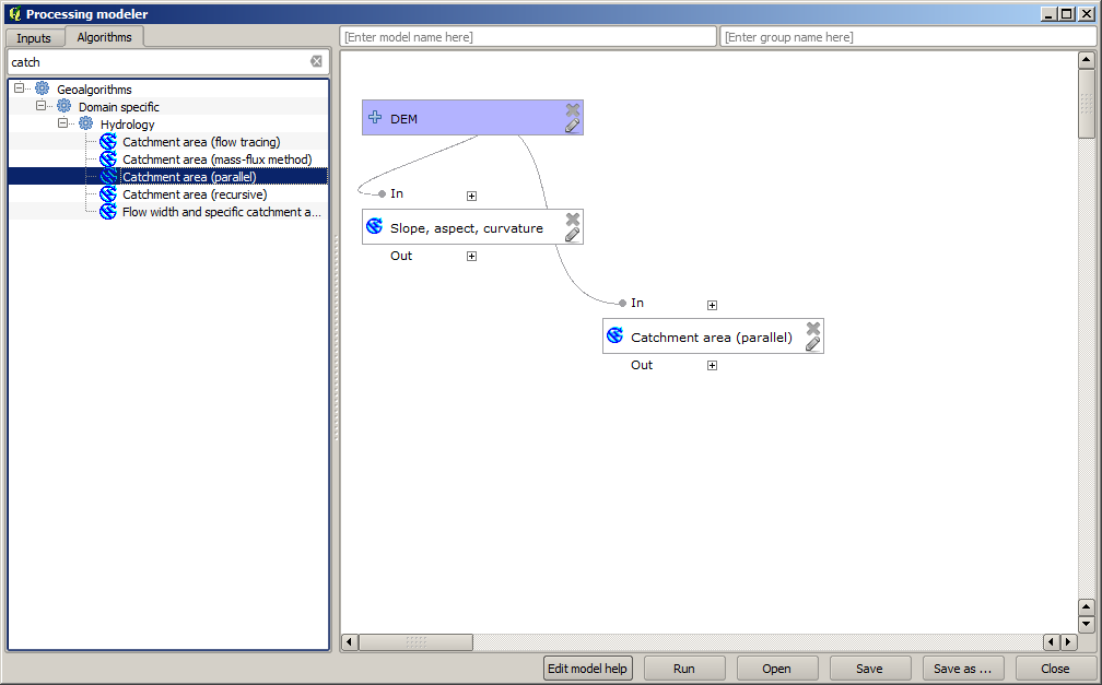
8. There is not much to select in this first dialog, since we do not have but just one layer in our model (The DEM input that we created). Actually, the default configuration of the dialog is the correct one in this case, so you just have to press OK. This is what you will now have in the modeler canvas.

   

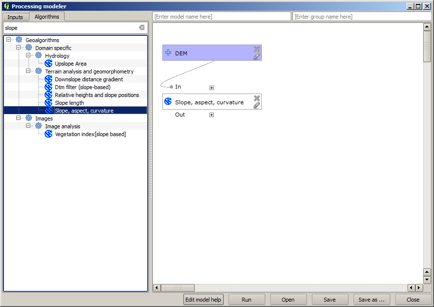
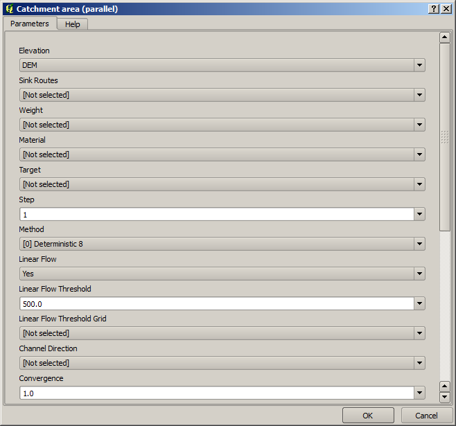
9. El segundo algoritmo tenemos que añadir a nuestro modelo esta el algoritmo de zona de captación. Nosotros utilizamos el algoritmo llamado Zona de captación (Paralelo). Utilizaremos la capa MDT de nuevo como entrada, y ninguno de los resultados producidos son finales, así que aquí es cómo se tiene que llenar el diálogo correspondiente.

   

   Agora o seu modelo deve estar semelhante a este.

   

10. The last step is to add the Topographic wetness index algorithm, with the following configuration.

    

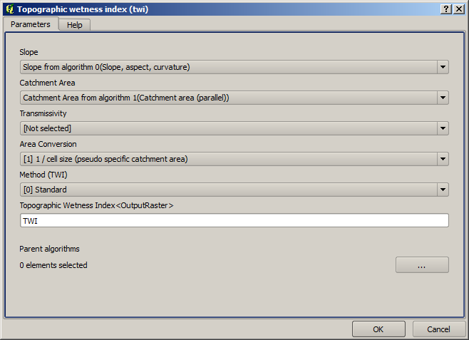
    En este caso, estaremos utilizando el MDT como entrada, pero en su lugar, utilizaremos la capa de pendiente y zona de captación que están calculadas por el algoritmo que previamente añadimos. A medida que agrega nuevos algoritmos, las salidas que producen estén disponibles para otros algoritmos, y su uso se vincula a los algoritmos, creando el flujo de trabajo.

11. In this case, the output TWI layer is a final layer, so we have to indicate so. In the corresponding textbox, enter the name that you want to be shown for this output.

    Ahora nuestro modelo esta terminada y debería tener este aspecto.

    

12. Inserir um nome e um nome de grupo na parte superior da janela do modelo.

    

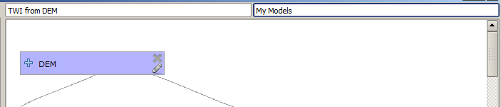
13. Save it clicking on the Save button. You can save it anywhere you want and open it later, but if you save it in the models folder (which is the folder that you will see when the save file dialog appears), your model will also be available in the toolbox as well. So stay on that folder and save the model with the filename that you prefer.

14. Now close the modeler dialog and go to the toolbox. In the Models entry you will find your model.

    

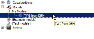
15. Você pode executá-lo como qualquer algoritmo normal, clicando duas vezes nele.

    

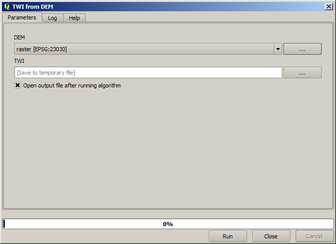
    Como se puede ver, el diálogo de parámetros, contiene la entrada que se añadió al modelo, junto con las salidas que se establecieron como finales al agregar los algoritmos correspondientes.

16. Ejecútelo utilizando el MDT como entrada y se obtendrá la capa TWI en solo un paso.