6.2. Lesson: Análise Vetorial

Vector data can also be analyzed to reveal how different features interact with each other in space. There are many different analysis-related functions, so we won’t go through them all. Rather, we will pose a question and try to solve it using the tools that QGIS provides.

O objetivo desta lição: Fazer uma pergunta e respondê-la usando ferramentas de análise.

6.2.1. O Processo SIG

Before we start, it would be useful to give a brief overview of a process that can be used to solve a problem. The way to go about it is:

1. Definir o Problema

2. Coletar os Dados

3. Analisar o Problema

4. Demonstrar os Resultados

6.2.2. O Problema

Comecemos o processo definindo o problema a ser solucionado. Por exemplo, você é um funcionário público e está procurando por propriedades residenciais em Swellendam por clientes que se encaixam nos seguintes critérios:

1. It needs to be in Swellendam

2. It must be within reasonable driving distance of a school (say 1km)

3. It must be more than 100m squared in size

4. A menos de 50m de uma estrada principal

5. A menos de 500m de um restaurante

6.2.3. Os Dados

To answer these questions, we are going to need the following data:

1. The residential properties (buildings) in the area

2. The roads in and around the town

3. The location of schools and restaurants

4. The size of buildings

These data are available through OSM, and you should find that the dataset you have been using throughout this manual also can be used for this lesson.

If you want to download data from another area, jump to the Introduction Chapter to read how to do it.

Nota

Aunque hay coherencia en los campos de datos que encontramos en las descargas de OSM, pueden variar en su cobertura y detalle. Si ves, por ejemplo, que la región que has elegido no contiene información sobre restaurantes, quizás necesitas elegir otra región.

6.2.4. Follow Along: Inicie um projeto e obtenha os dados

We first need to load the data to work with.

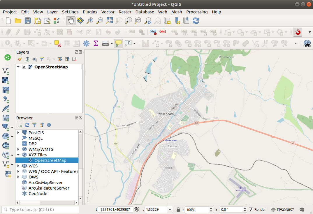
1. Inicie um novo projeto QGIS

2. If you want, you can add a background map. Open the Browser and load the OSM background map from the XYZ Tiles menu.

   

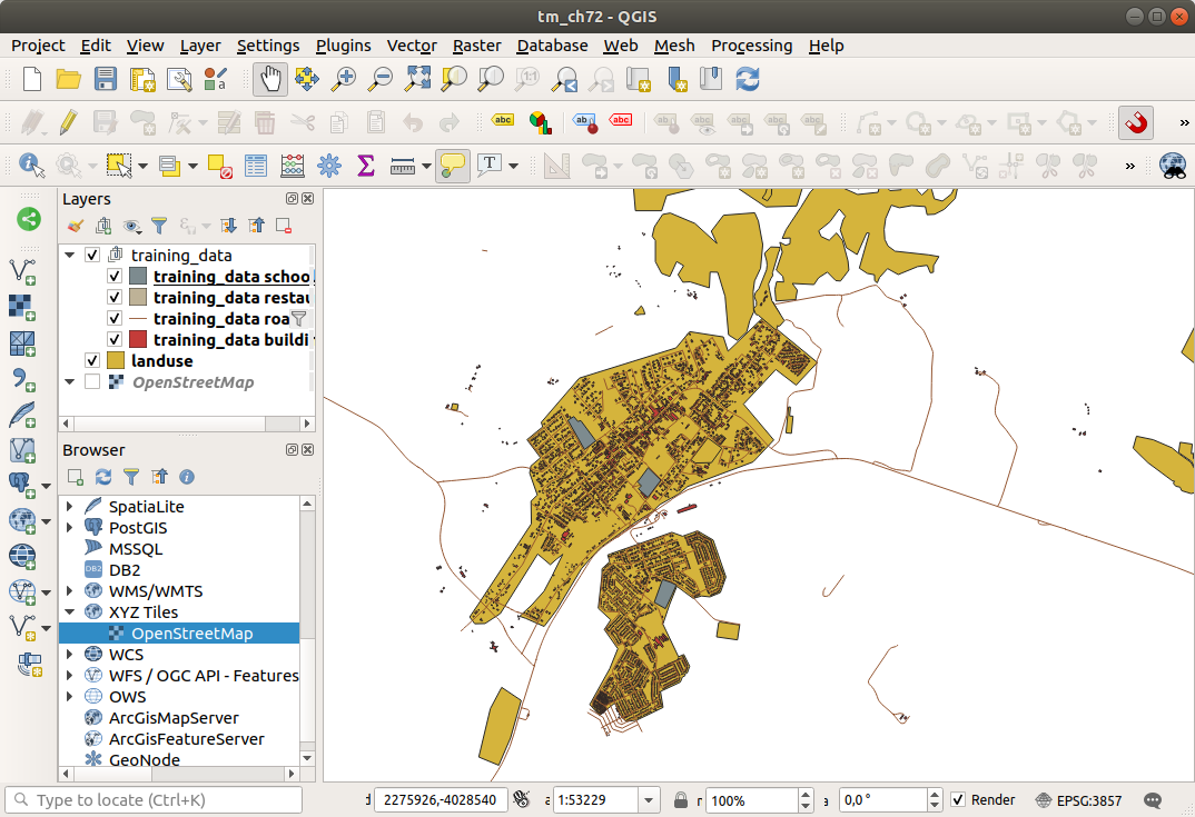
3. In the training_data.gpkg Geopackage database, you will find most the datasets we will use in this chapter:

   1. buildings

   2. roads

   3. restaurantes

   4. schools

   Load them, and also landuse.sqlite.

4. Zoom to the layer extent to see Swellendam, South Africa

   Before proceeding we will filter the roads layer, in order to have only some specific road types to work with.

   Some roads in OSM datasets are listed as unclassified, tracks, path and footway. We want to exclude these from our dataset and focus on the other road types, more suitable for this exercise.

   Moreover, OSM data might not be updated everywhere, and we will also exclude NULL values.

5. Right click on the roads layer and choose Filter….

6. In the dialog that pops up we filter these features with the following expression:

   "highway" NOT IN ('footway', 'path', 'unclassified', 'track') AND "highway" IS NOT NULL
   

   The concatenation of the two operators NOT and IN excludes all the features that have these attribute values in the highway field.

   IS NOT NULL combined with the AND operator excludes roads with no value in the highway field.

   Note the icon next to the roads layer. It helps you remember that this layer has a filter activated, so some features may not be available in the project.

O mapa com todos os dados deve se parecer com o seguinte:

6.2.5. Try Yourself Converter SRC de camadas

Como vamos medir distâncias dentro de nossas camadas, precisamos alterar o SRC das camadas. Para fazer isso, precisamos selecionar cada camada por vez, salvar a camada em uma nova com nossa nova projeção e importar essa nova camada para o nosso mapa.

You have many different options, e.g. you can export each layer as an ESRI Shapefile format dataset, you can append the layers to an existing GeoPackage file, or you can create another GeoPackage file and fill it with the new reprojected layers. We will show the last option, so the training_data.gpkg will remain clean. Feel free to choose the best workflow for yourself.

Nota

In this example, we are using the WGS 84 / UTM zone 34S CRS, but you should use a UTM CRS which is more appropriate for your region.

1. Right click the roads layer in the Layers panel

2. Click Export –> Save Features As…

3. In the Save Vector Layer As dialog choose GeoPackage as Format

4. Click on … for the File name, and name the new GeoPackage vector_analysis

5. Change the Layer name to roads_34S

6. Change the CRS to WGS 84 / UTM zone 34S

7. Click on OK:

   

   This will create the new GeoPackage database and add the roads_34S layer.

8. Repeat this process for each layer, creating a new layer in the vector_analysis.gpkg GeoPackage file with _34S appended to the original name and removing each of the old layers from the project.

   Nota

   When you choose to save a layer to an existing GeoPackage, QGIS will append that layer to the GeoPackage.

9. Once you have completed the process for all the layers, right click on any layer and click Zoom to layer extent to focus the map to the area of interest.

Now that we have converted OSM data to a UTM projection, we can begin our calculations.

6.2.6. Follow Along: Analizando el Problema: Distancias Desde Colegios y Carreteras.

QGIS allows you to calculate distances between any vector object.

1. Make sure that only the roads_34S and buildings_34S layers are visible (to simplify the map while you’re working)

2. Click on the Processing ► Toolbox to open the analytical core of QGIS. Basically, all algorithms (for vector and raster analysis) are available in this toolbox.

3. We start by calculating the area around the roads_34S by using the Buffer algorithm. You can find it in the Vector Geometry group.

   

   Or you can type buffer in the search menu in the upper part of the toolbox: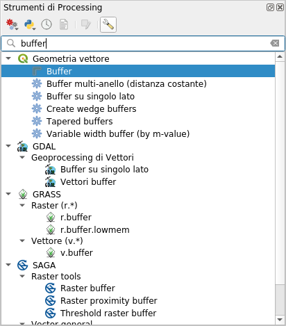

   

4. Clique duas vezes nele para abrir a caixa de diálogo do algoritmo

5. Select roads_34S as Input layer, set Distance to 50 and use the default values for the rest of the parameters.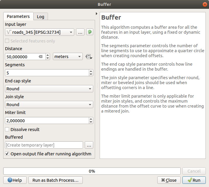

   

6. The default Distance is in meters because our input dataset is in a Projected Coordinate System that uses meter as its basic measurement unit. You can use the combo box to choose other projected units like kilometers, yards, etc.

   Nota

   If you are trying to make a buffer on a layer with a Geographical Coordinate System, Processing will warn you and suggest to reproject the layer to a metric Coordinate System.

7. By default, Processing creates temporary layers and adds them to the Layers panel. You can also append the result to the GeoPackage database by:

   1. Clicking on the … button and choose Save to GeoPackage…

   2. Naming the new layer roads_buffer_50m

   3. Saving it in the vector_analysis.gpkg file

   

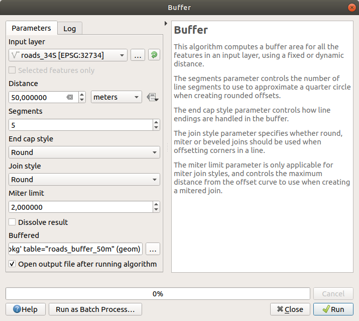
8. Click on Run, and then close the Buffer dialog

   Ahora tu mapa se parece un poco a esto:

   

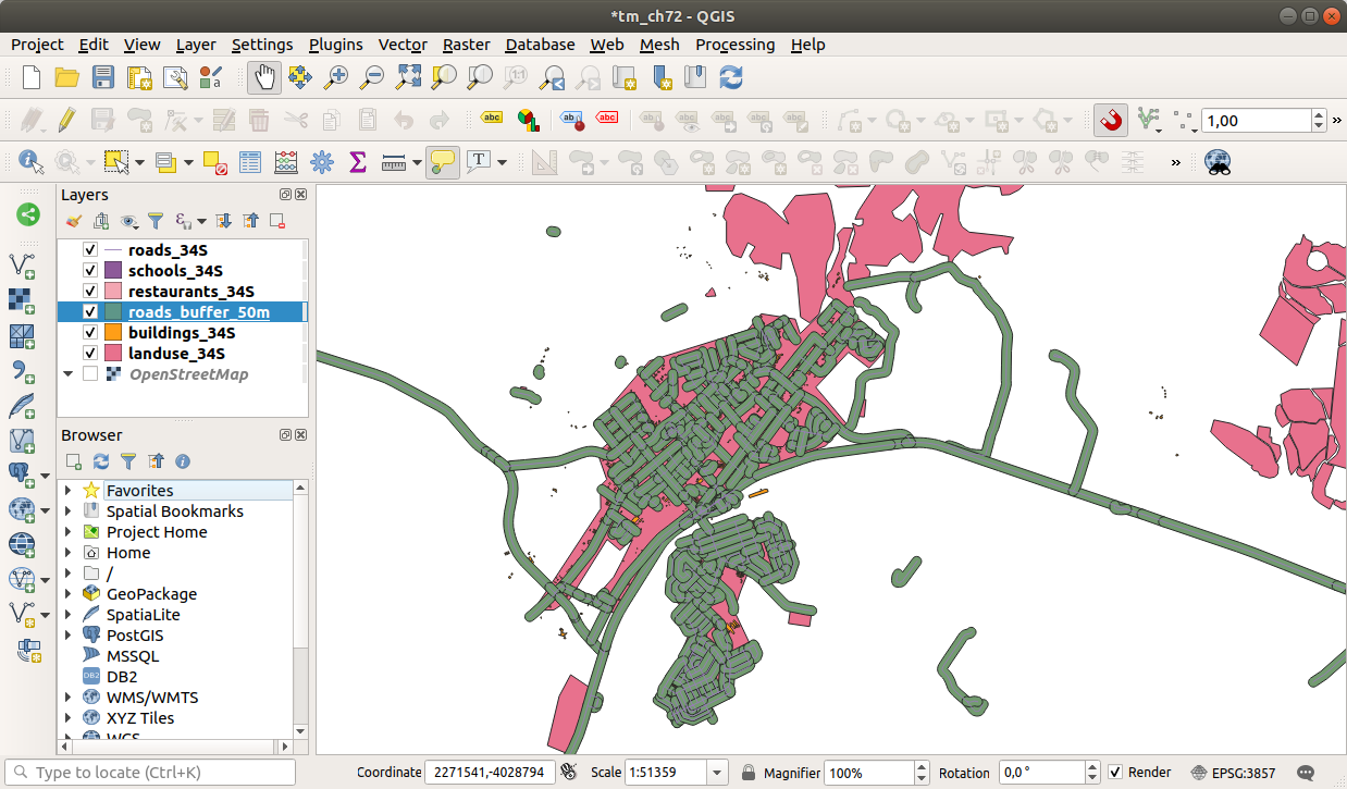
If your new layer is at the top of the Layers list, it will probably obscure much of your map, but this gives you all the areas in your region which are within 50m of a road.

Notice that there are distinct areas within your buffer, which correspond to each individual road. To get rid of this problem:

1. Uncheck the roads_buffer_50m layer and re-create the buffer with Dissolve results enabled.

   

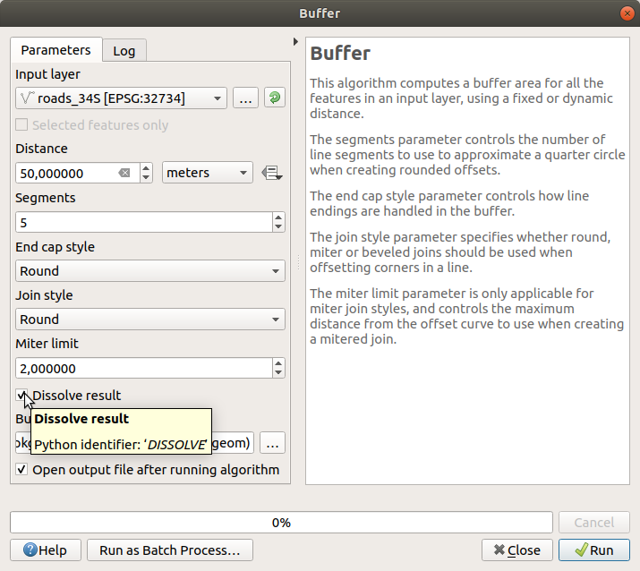
2. Save the output as roads_buffer_50m_dissolved

3. Click Run and close the Buffer dialog

Once you have added the layer to the Layers panel, it will look like this:

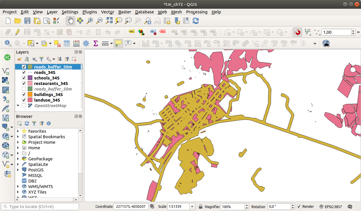
Ahora no hay subdivisiones innecesarias.

Nota

The Short Help on the right side of the dialog explains how the algorithm works. If you need more information, just click on the Help button in the bottom part to open a more detailed guide of the algorithm.

6.2.7. Try Yourself Distancia desde colegios.

Usa el mismo enfoque que anteriormente y crea un buffer para tus colegios.

It shall to be 1 km in radius. Save the new layer in the vector_analysis.gpkg file as schools_buffer_1km_dissolved.

Comprueba tus resultados

6.2.8. Follow Along: Areas que se sobrepõe.

Now we have identified areas where the road is less than 50 meters away and areas where there is a school within 1 km (direct line, not by road). But obviously, we only want the areas where both of these criteria are satisfied. To do that, we will need to use the Intersect tool. You can find it in Vector Overlay group in the Processing Toolbox.

1. Use the two buffer layers as Input layer and Overlay layer, choose vector_analysis.gpkg GeoPackage in Intersection with Layer name road_school_buffers_intersect. Leave the rest as suggested (default).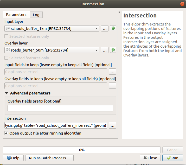

   

2. Haz clic en Run.

   In the image below, the blue areas are where both of the distance criteria are satisfied.

   

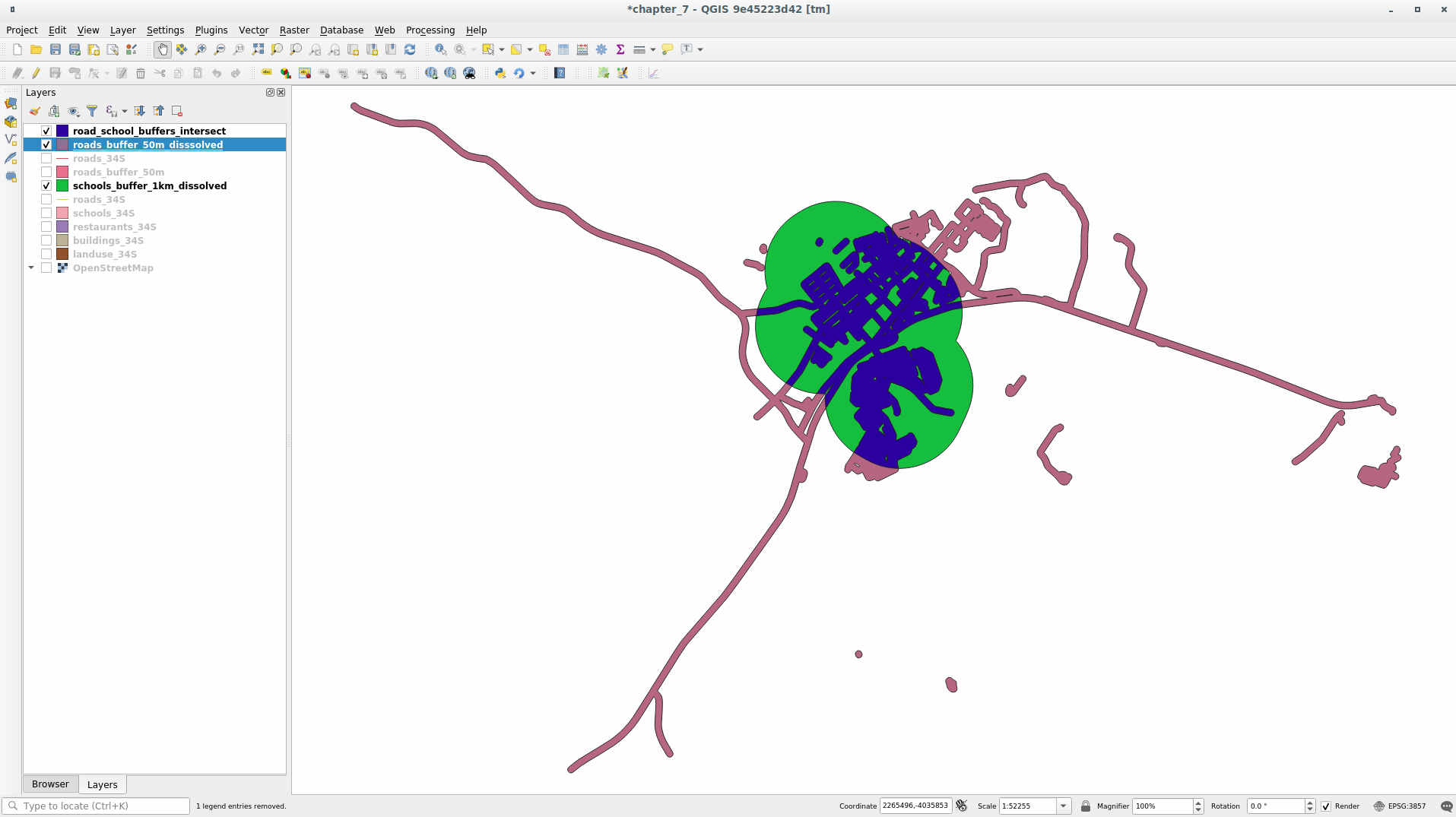
3. Usted puede borrar las dos capas buffer y solo mantener la que muestra la superposición, dado que eso era lo que queriamos conocer en primer lugar:

   

6.2.9. Follow Along: Extract the Buildings

Agora você tem a área em que as construções devem se sobrepor. Em seguida, você deseja extrair as construções nessa área.

1. Look for the menu entry Vector Selection ► Extract by location within the Processing Toolbox

2. Select buildings_34S in Extract features from. Check intersect in Where the features (geometric predicate), select the buffer intersection layer in By comparing to the features from. Save to the vector_analysis.gpkg, and name the layer well_located_houses.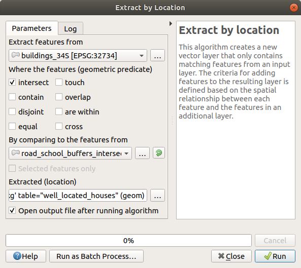

   

3. Click Run and close the dialog

4. You will probably find that not much seems to have changed. If so, move the well_located_houses layer to the top of the layers list, then zoom in.

   

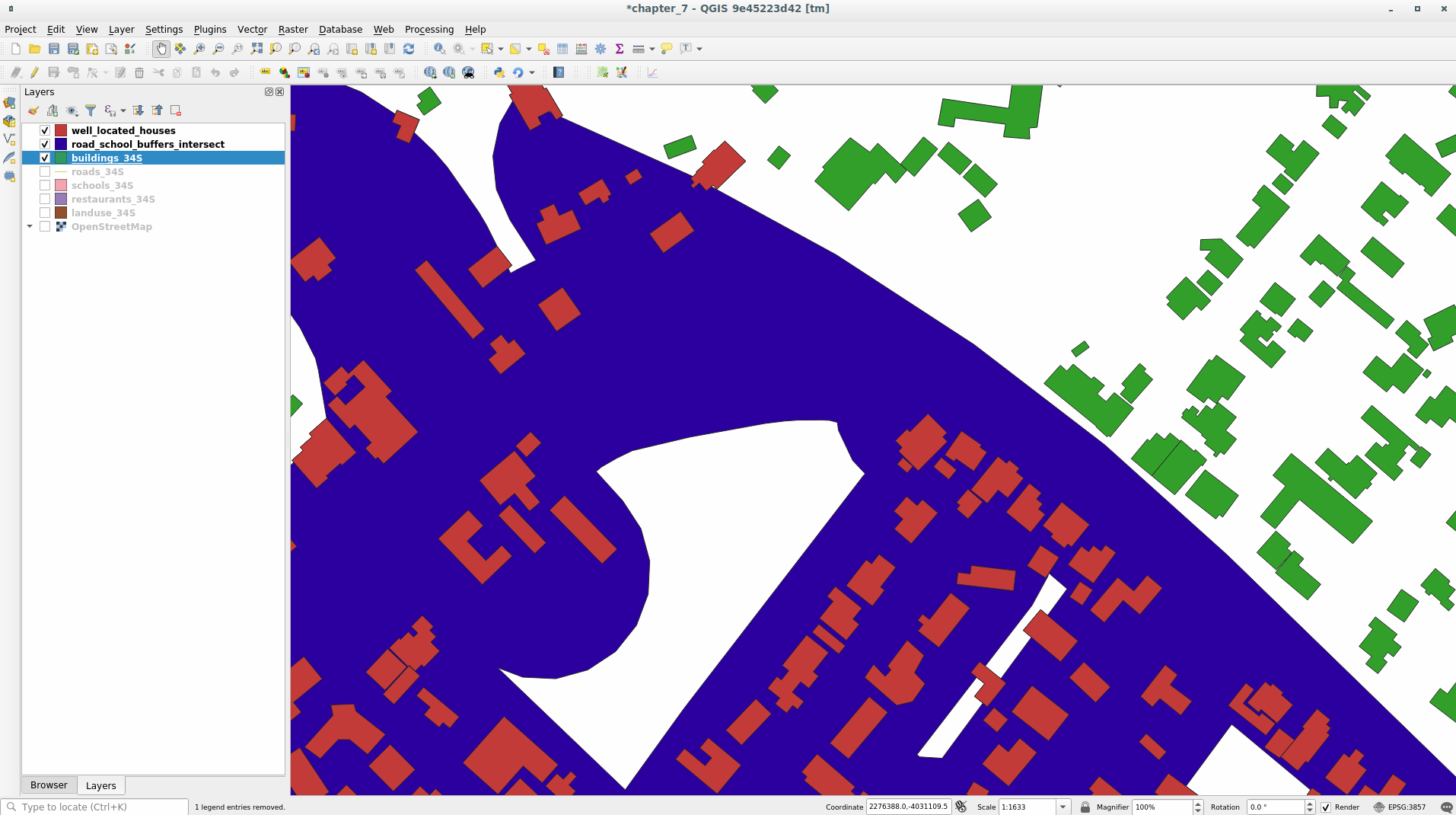
   Os prédios vermelhos são aqueles que atendem aos nossos critérios, enquanto os prédios em verde são aqueles que não atendem.

5. Now you have two separated layers and can remove buildings_34S from the layer list.

6.2.10. Try Yourself Filtrado adicional de nuestros Edificios

Ahora tenemos una capa que nos muestra los edificios en un radio de 1km de una escuela y a menos de 50m de una carretera. Ahora tenemos que reducir la selección para que sólo nos muestre los edificios que están a menos de 500 metros de un restaurante.

Usando os processos descritos acima, crie uma nova camada chamada casas_restaurantes_500m, que filtra ainda mais a sua camada casas_bem_localizadas para mostrar apenas aqueles que estão a 500m de um restaurante.

:ref:` Comprueba tus resultados <vector-analysis-basic-2>`

6.2.11. Follow Along: Seleccione las Construcciones de Tamaño Adecuado

To see which buildings are of the correct size (more than 100 square meters), we need to calculate their size.

1. Select the houses_restaurants_500m layer and open the Field Calculator by clicking on the ^{Open Field Calculator} button in the main toolbar or in the attribute table window

2. Select Create a new field, set the Output field name to AREA, choose Decimal number (real) as Output field type, and choose $area from the Geome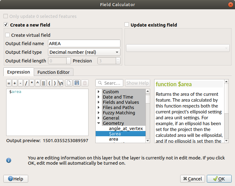try group.

   

   The new field AREA will contain the area of each building in square meters.

3. Click OK. The AREA field has been added at the end of the attribute table.

4. Click the ^{Toggle Editing} button to finish editing, and save your edits when prompted.

5. In the Source tab of the layer properties, set the Provider Feature Filter to "AREA >= 100.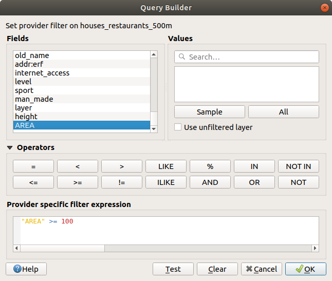

   

6. Haz clic en OK.

Your map should now only show you those buildings which match our starting criteria and which are more than 100 square meters in size.

6.2.12. Try Yourself

Save your solution as a new layer, using the approach you learned above for doing so. The file should be saved within the same GeoPackage database, with the name solution.

6.2.13. In Conclusion

Using the GIS problem solving approach together with QGIS vector analysis tools, you were able to solve a problem with multiple criteria quickly and easily.

6.2.14. What’s Next?

In the next lesson, we will look at how to calculate the shortest distance along roads from one point to another.