Importante
A tradução é um esforço comunitário você pode contribuir. Esta página está atualmente traduzida em 39.13%.
6.2. Lesson: Vector Analysis
Vector data can also be analyzed to reveal how different features interact with each other in space. There are many different analysis-related functions, so we won’t go through them all. Rather, we will pose a question and try to solve it using the tools that QGIS provides.
O objetivo desta lição: Fazer uma pergunta e respondê-la usando ferramentas de análise.
6.2.1. ★☆☆ The GIS Process
Antes de começarmos, seria útil dar uma breve visão geral de um processo que pode ser usado para resolver um problema. A maneira de fazer isso é:
Definir o Problema
Coletar os Dados
Analisar o Problema
Demonstrar os Resultados
6.2.2. ★☆☆ The Problem
Comecemos o processo definindo o problema a ser solucionado. Por exemplo, você é um funcionário público e está procurando por propriedades residenciais em Swellendam por clientes que se encaixam nos seguintes critérios:
It needs to be in Swellendam
Deve estar a uma distância razoável de uma escola (digamos 1 km)
Deve ter mais de 100m quadrados de tamanho
A menos de 50m de uma estrada principal
A menos de 500m de um restaurante
6.2.3. ★☆☆ The Data
Para responder a essas perguntas, vamos precisar dos seguintes dados:
As propriedades residenciais (edifícios) na área
As estradas dentro e ao redor da cidade
A localização de escolas e restaurantes
O tamanho dos prédios
These data are available through OSM, and you should find that the dataset you have been using throughout this manual also can be used for this lesson.
If you want to download data from another area, jump to the Introduction Chapter to read how to do it.
Nota
Aunque hay coherencia en los campos de datos que encontramos en las descargas de OSM, pueden variar en su cobertura y detalle. Si ves, por ejemplo, que la región que has elegido no contiene información sobre restaurantes, quizás necesitas elegir otra región.
6.2.4. ★☆☆ Follow Along: Start a Project and get the Data
Primeiro precisamos carregar os dados para trabalhar.
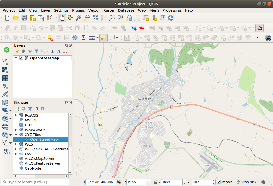
Inicie um novo projeto QGIS
If you want, you can add a background map. Open the Browser and load the OSM background map from the XYZ Tiles menu.
In the
training_data.gpkgGeopackage database, you will find most the datasets we will use in this chapter:buildingsroadsrestaurantsschools
Load them, and also
landuse.sqlite.Zoom to the layer extent to see Swellendam, South Africa
Before proceeding we will filter the
roadslayer, in order to have only some specific road types to work with.Some roads in OSM datasets are listed as
unclassified,tracks,pathandfootway. We want to exclude these from our dataset and focus on the other road types, more suitable for this exercise.Moreover, OSM data might not be updated everywhere, and we will also exclude
NULLvalues.Right click on the
roadslayer and choose Filter….Na caixa de diálogo exibida, filtramos essas feições com a seguinte expressão:
"highway" NOT IN ('footway', 'path', 'unclassified', 'track') AND "highway" IS NOT NULL
The concatenation of the two operators
NOTandINexcludes all the features that have these attribute values in thehighwayfield.IS NOT NULLcombined with theANDoperator excludes roads with no value in thehighwayfield.Note the
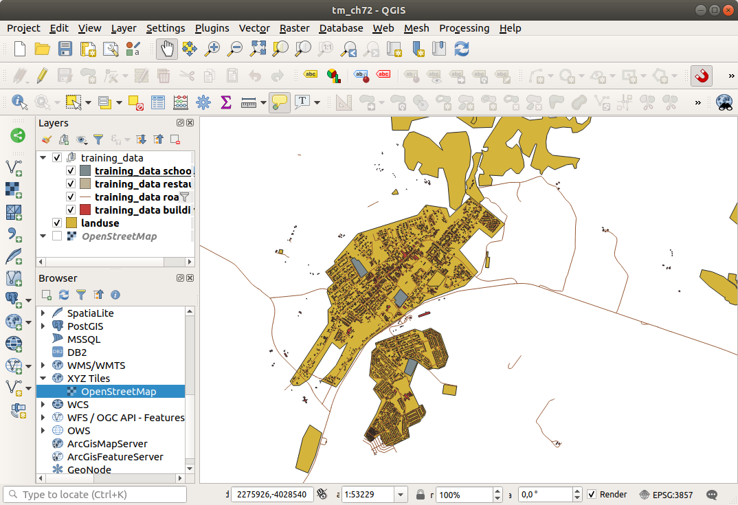
 icon next to the
 roadslayer. It helps you remember that this layer has a filter activated, so some features may not be available in the project.
O mapa com todos os dados deve se parecer com o seguinte:
6.2.5. ★☆☆ Try Yourself: Convert Layers’ CRS
Como vamos medir distâncias dentro de nossas camadas, precisamos alterar o SRC das camadas. Para fazer isso, precisamos selecionar cada camada por vez, salvar a camada em uma nova com nossa nova projeção e importar essa nova camada para o nosso mapa.
You have many different options, e.g. you can export each layer as an
ESRI Shapefile format dataset, you can append the layers to an
existing GeoPackage file, or you can create another GeoPackage file
and fill it with the new reprojected layers.
We will show the last option, so the training_data.gpkg will
remain clean.
Feel free to choose the best workflow for yourself.
Nota
In this example, we are using the WGS 84 / UTM zone 34S CRS, but you should use a UTM CRS which is more appropriate for your region.
Right click the
roadslayer in the Layers panelClick Export –> Save Features As…
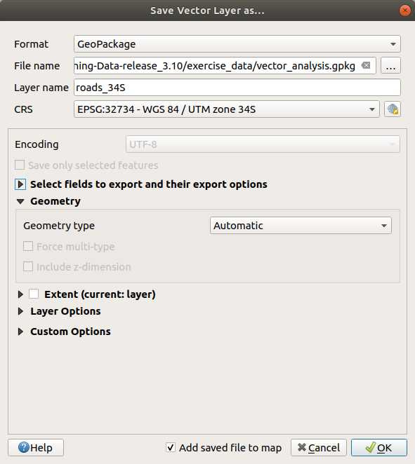
In the Save Vector Layer As dialog choose GeoPackage as Format
Click on … for the File name, and name the new GeoPackage
vector_analysisChange the Layer name to
roads_34SChange the CRS to WGS 84 / UTM zone 34S
Click on OK:
This will create the new GeoPackage database and add the
roads_34Slayer.Repeat this process for each layer, creating a new layer in the
vector_analysis.gpkgGeoPackage file with_34Sappended to the original name.On macOS, press the Replace button in the dialog that pops up to allow QGIS to overwrite the existing GeoPackage.
Nota
When you choose to save a layer to an existing GeoPackage, QGIS will add that layer next to the existing layers in the GeoPackage, if no layer of the same name already exists.
Remove each of the old layers from the project
Once you have completed the process for all the layers, right click on any layer and click Zoom to layer extent to focus the map to the area of interest.
Now that we have converted OSM data to a UTM projection, we can begin our calculations.
6.2.6. ★☆☆ Follow Along: Analyzing the Problem: Distances From Schools and Roads
O QGIS permite calcular distâncias entre qualquer objeto vetorial.
Make sure that only the
roads_34Sandbuildings_34Slayers are visible (to simplify the map while you’re working)Click on the to open the analytical core of QGIS. Basically, all algorithms (for vector and raster analysis) are available in this toolbox.
We start by calculating the area around the
roads_34Sby using the Buffer algorithm. You can find it in the group.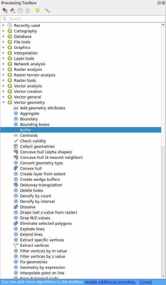
Or you can type
bufferin the search menu in the upper part of the toolbox: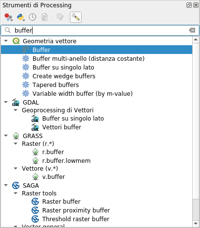
Clique duas vezes nele para abrir a caixa de diálogo do algoritmo
Select
roads_34Sas Input layer, set Distance to 50 and use the default values for the rest of the parameters.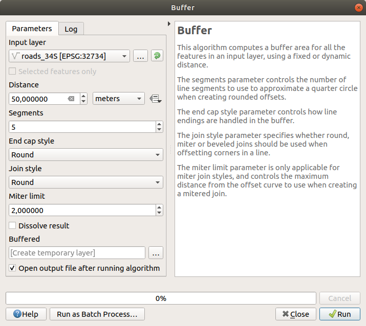
The default Distance is in meters because our input dataset is in a Projected Coordinate System that uses meter as its basic measurement unit. You can use the combo box to choose other projected units like kilometers, yards, etc.
Nota
If you are trying to make a buffer on a layer with a Geographical Coordinate System, Processing will warn you and suggest to reproject the layer to a metric Coordinate System.
By default, Processing creates temporary layers and adds them to the Layers panel. You can also append the result to the GeoPackage database by:
Clicking on the … button and choose Save to GeoPackage…
Naming the new layer
roads_buffer_50mSaving it in the
vector_analysis.gpkgfile
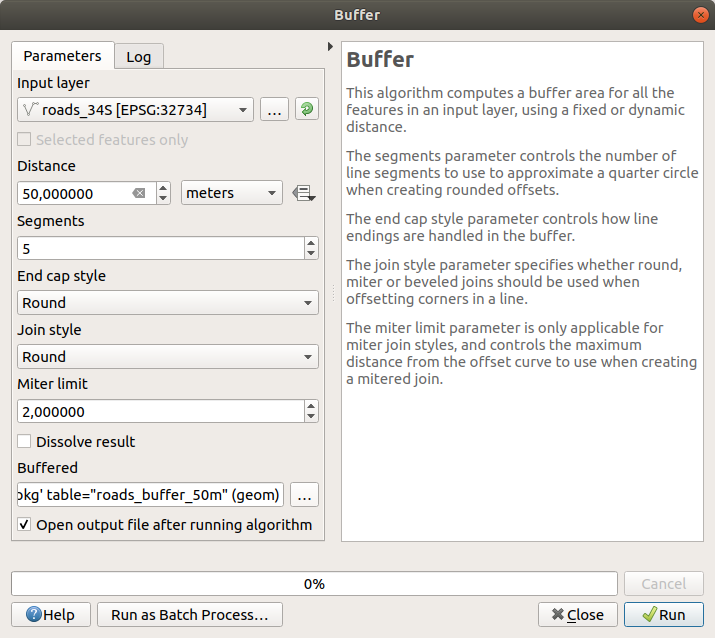
Click on Run, and then close the Buffer dialog
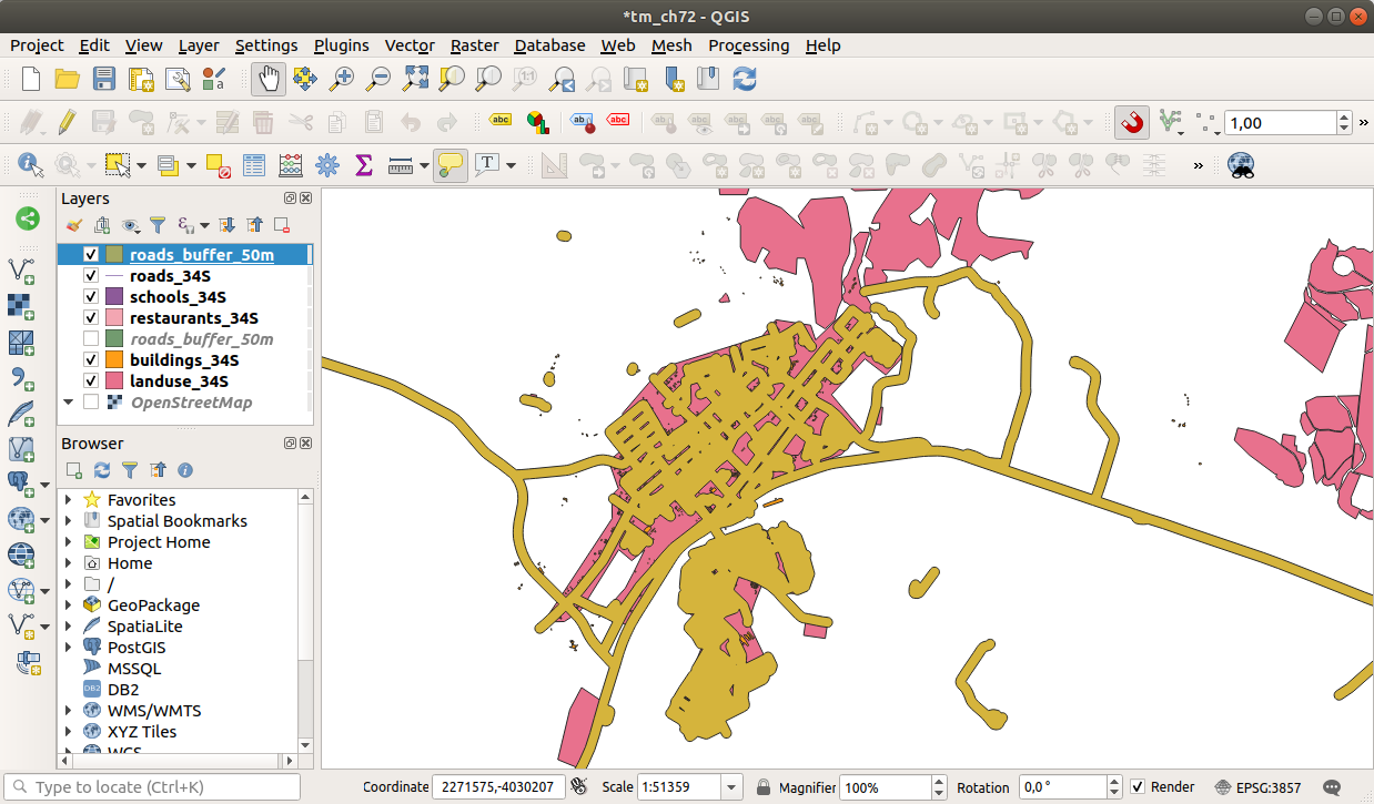
Ahora tu mapa se parece un poco a esto:
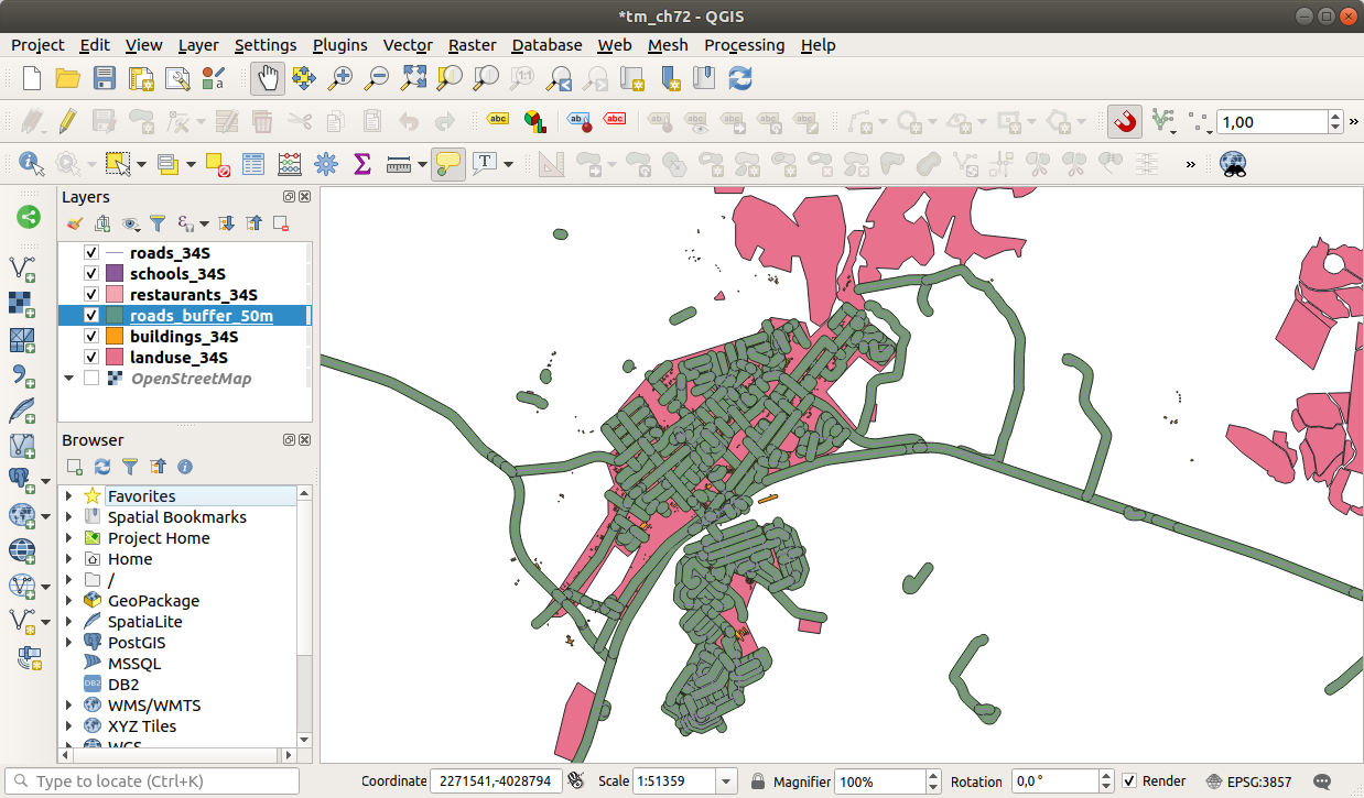
If your new layer is at the top of the Layers list, it will probably obscure much of your map, but this gives you all the areas in your region which are within 50m of a road.
Notice that there are distinct areas within your buffer, which correspond to each individual road. To get rid of this problem:
Uncheck the
roads_buffer_50mlayer and re-create the buffer with Dissolve results enabled.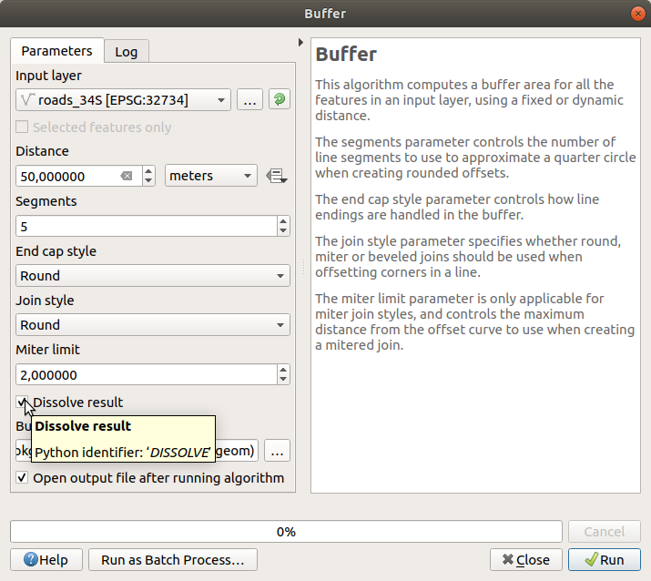
Save the output as
roads_buffer_50m_dissolvedClick Run and close the Buffer dialog
Once you have added the layer to the Layers panel, it will look like this:
Ahora no hay subdivisiones innecesarias.
Nota
The Short Help on the right side of the dialog explains how the algorithm works. If you need more information, just click on the Help button in the bottom part to open a more detailed guide of the algorithm.
6.2.7. ★☆☆ Try Yourself: Distance from schools
Usa el mismo enfoque que anteriormente y crea un buffer para tus colegios.
It shall be 1 km in radius.
Save the new layer in the vector_analysis.gpkg file as schools_buffer_1km_dissolved.
Responda
Your buffer dialog should look like this:
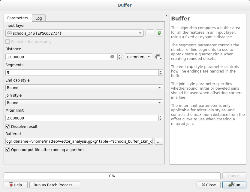
The Buffer distance is 1 kilometer.
The Segments to approximate value is set to
20. This is optional, but it’s recommended, because it makes the output buffers look smoother. Compare this: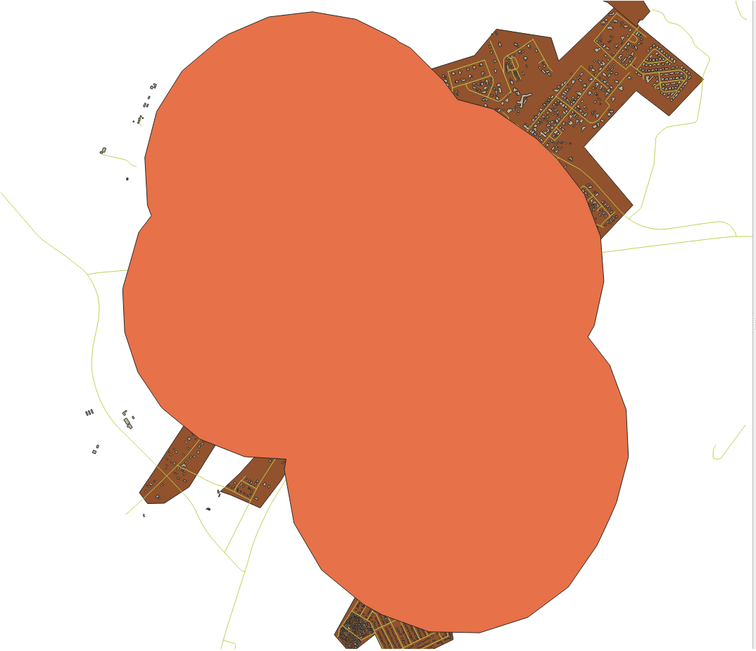
Para isso:
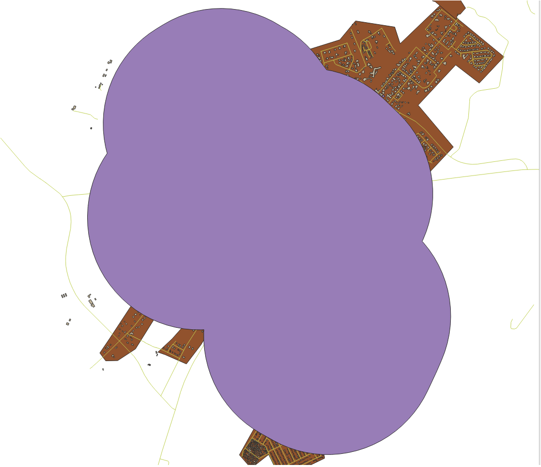
The first image shows the buffer with the Segments to approximate
value set to 5 and the second shows the value set to 20.
In our example, the difference is subtle, but you can see that the buffer’s edges
are smoother with the higher value.
6.2.8. ★☆☆ Follow Along: Overlapping Areas
Now we have identified areas where the road is less than 50 meters away and areas where there is a school within 1 km (direct line, not by road). But obviously, we only want the areas where both of these criteria are satisfied. To do that, we will need to use the Intersect tool. You can find it in group in the Processing Toolbox.
Use the two buffer layers as Input layer and Overlay layer, choose
vector_analysis.gpkgGeoPackage in Intersection with Layer nameroad_school_buffers_intersect. Leave the rest as suggested (default).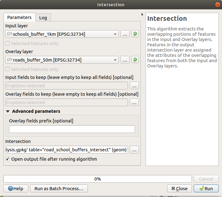
Haz clic en Run.
Na imagem abaixo, as áreas azuis são onde ambos os critérios de distância são satisfeitos.
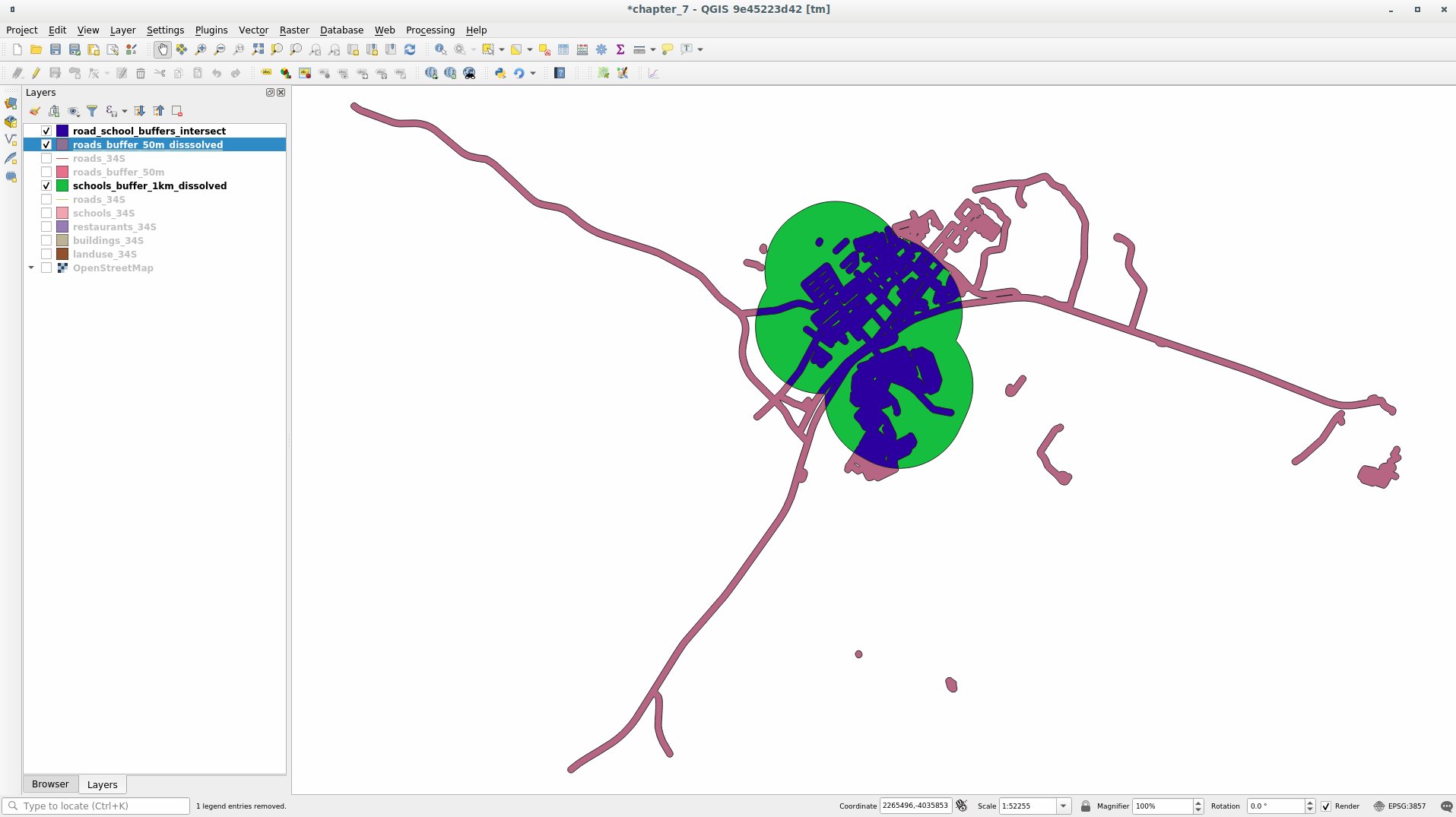
Usted puede borrar las dos capas buffer y solo mantener la que muestra la superposición, dado que eso era lo que queriamos conocer en primer lugar:
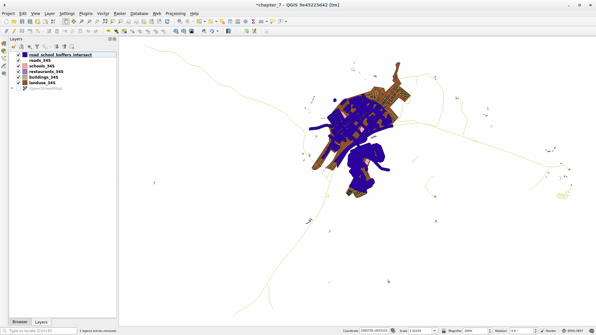
6.2.9. ★☆☆ Follow Along: Extract the Buildings
Agora você tem a área em que as construções devem se sobrepor. Em seguida, você deseja extrair as construções nessa área.
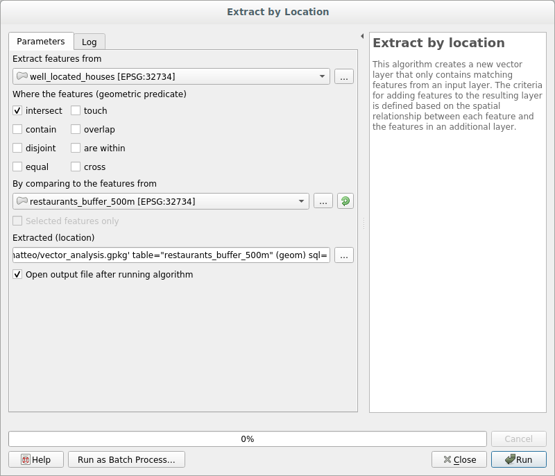
Look for the menu entry within the Processing Toolbox
Select
buildings_34Sin Extract features from. Check intersect in Where the features (geometric predicate), select the buffer intersection layer in By comparing to the features from. Save to thevector_analysis.gpkg, and name the layerwell_located_houses.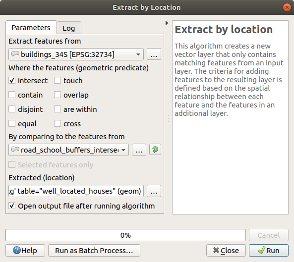
Click Run and close the dialog
You will probably find that not much seems to have changed. If so, move the
well_located_houseslayer to the top of the layers list, then zoom in.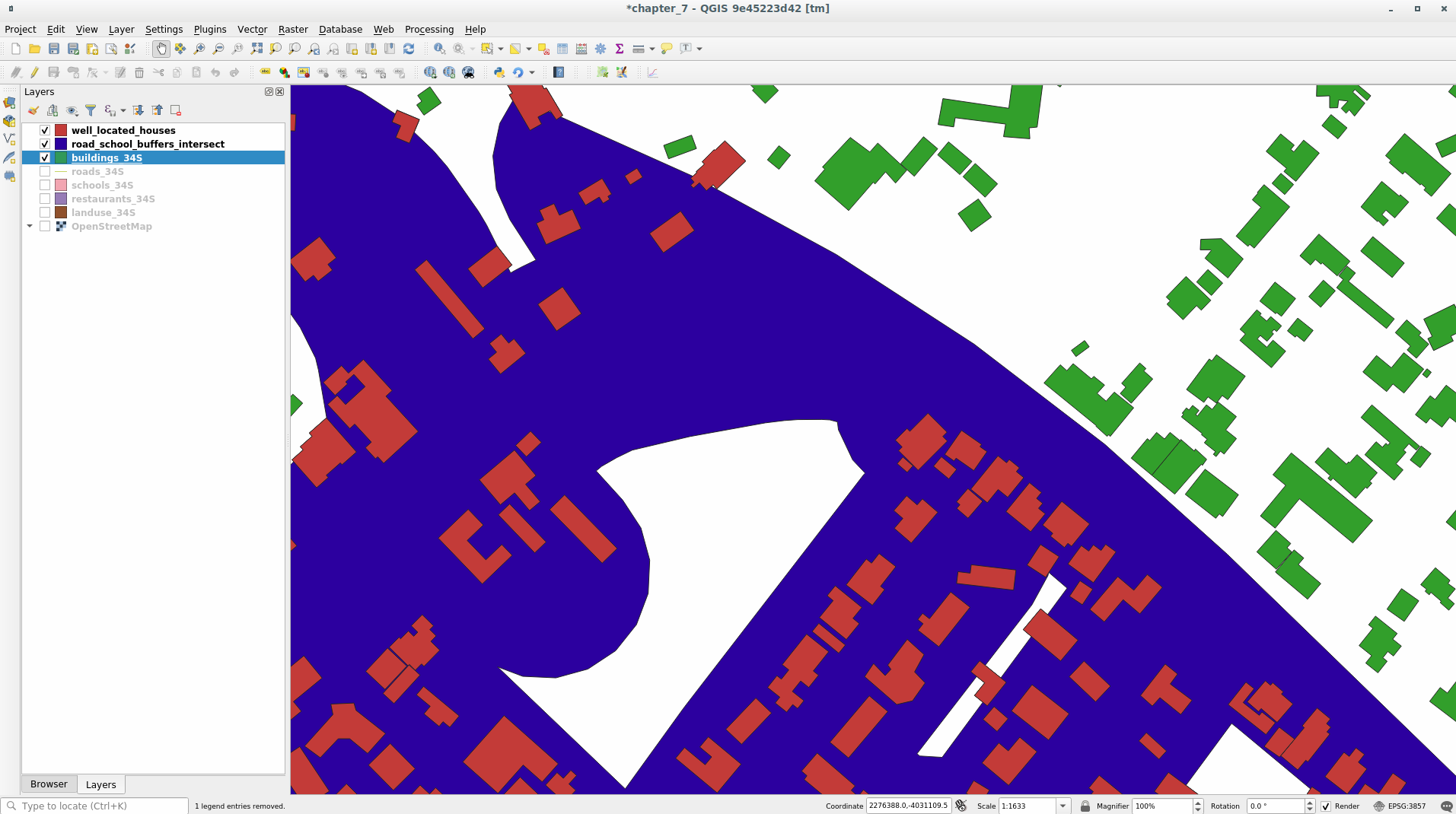
Os prédios vermelhos são aqueles que atendem aos nossos critérios, enquanto os prédios em verde são aqueles que não atendem.
Now you have two separated layers and can remove
buildings_34Sfrom the layer list.
6.2.10. ★★☆ Try Yourself: Further Filter our Buildings
Ahora tenemos una capa que nos muestra los edificios en un radio de 1km de una escuela y a menos de 50m de una carretera. Ahora tenemos que reducir la selección para que sólo nos muestre los edificios que están a menos de 500 metros de un restaurante.
Using the processes described above, create a new layer called
houses_restaurants_500m which further filters your
well_located_houses layer to show only those which are
within 500m of a restaurant.
Responda
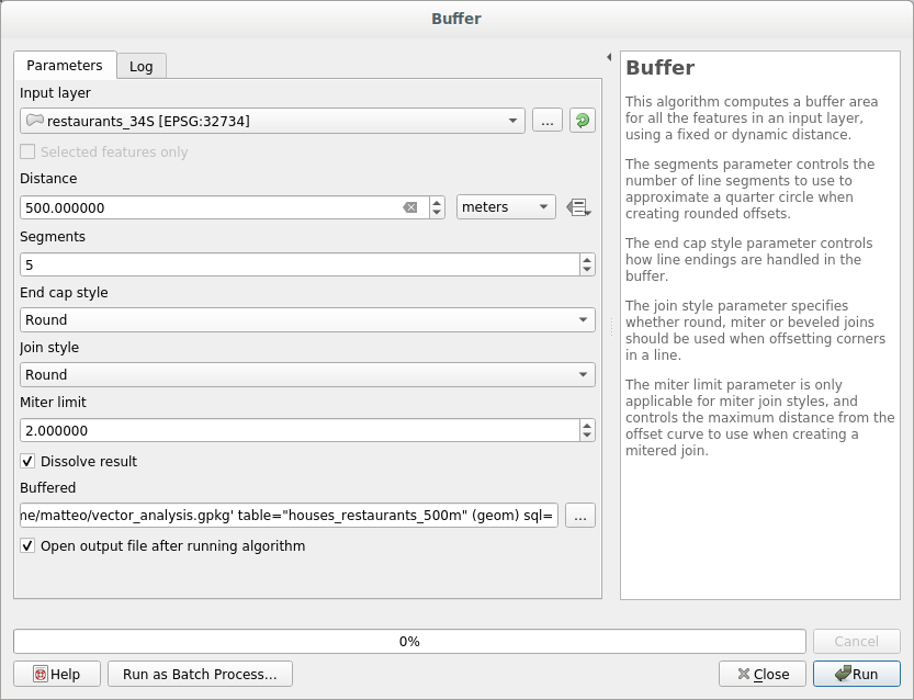
To create the new houses_restaurants_500m layer, we go through a two step
process:
Primeiro, criar um buffer de 500m ao redor dos restaurantes e adicionar a camada ao mapa:
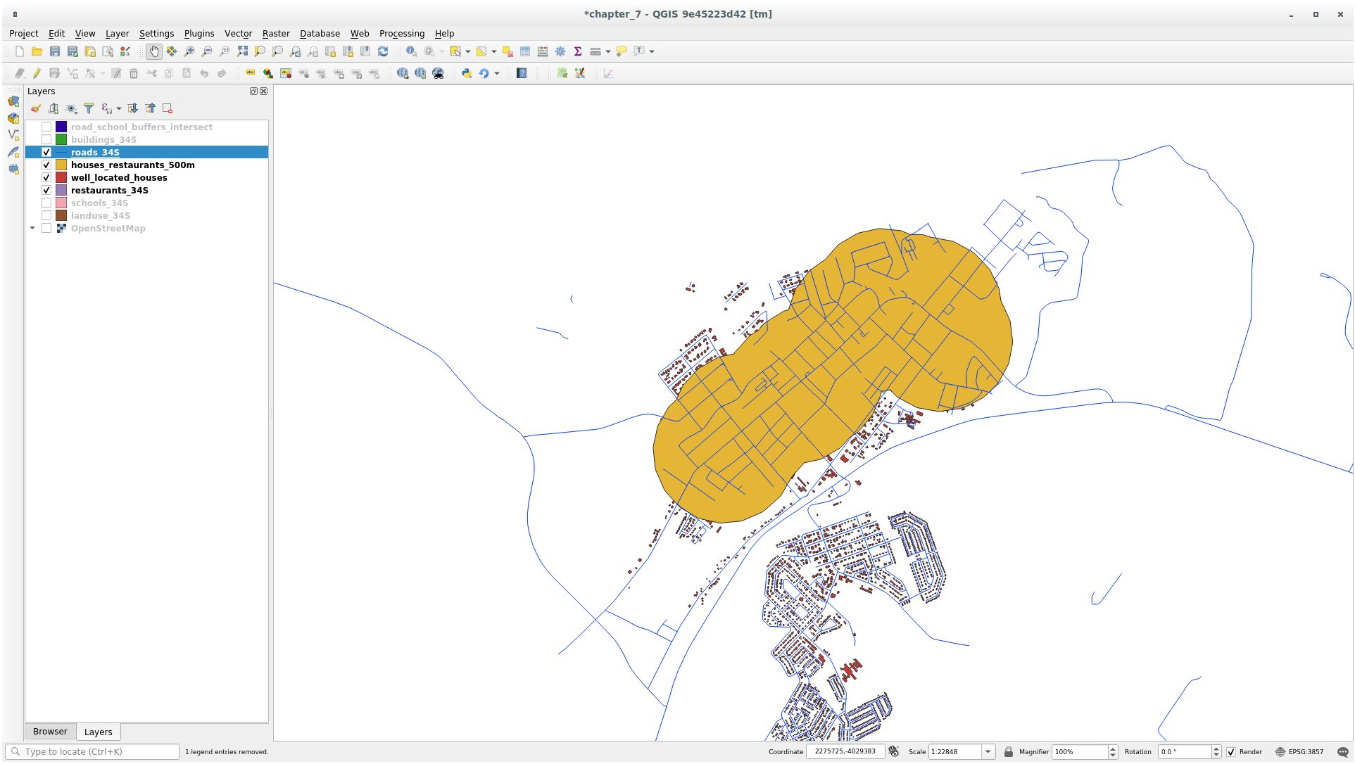
Em seguida, extrair edifícios dentro dessa área de buffer:
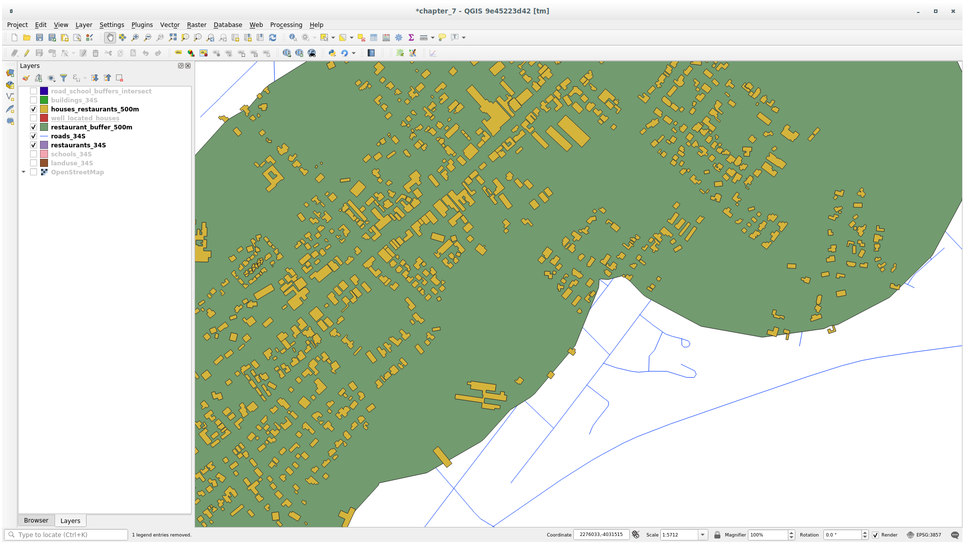
Seu mapa agora deve mostrar apenas os prédios que estão a 50m de uma estrada, 1km de uma escola e 500m de um restaurante:
6.2.11. ★☆☆ Follow Along: Select Buildings of the Right Size
Para ver quais edifícios são do tamanho correto (mais de 100 metros quadrados), precisamos calcular seu tamanho.
Select the
houses_restaurants_500mlayer and open the Field Calculator by clicking on the Open Field Calculator button in the main toolbar or in
the attribute table window
Open Field Calculator button in the main toolbar or in
the attribute table windowSelect Create a new field, set the Output field name to
AREA, choose Decimal number (real) as Output field type, and choose$areafrom the group.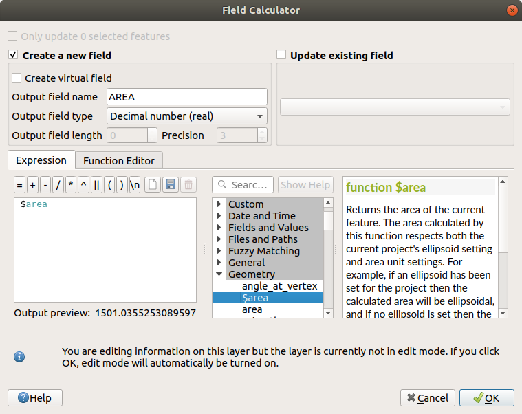
O novo campo
AREAconterá a área de cada edifício em metros quadrados.Click OK. The
AREAfield has been added at the end of the attribute table.Click the
 Toggle Editing button to finish
editing, and save your edits when prompted.
Toggle Editing button to finish
editing, and save your edits when prompted.In the tab of the layer properties, set the Provider Feature Filter to
"AREA >= 100.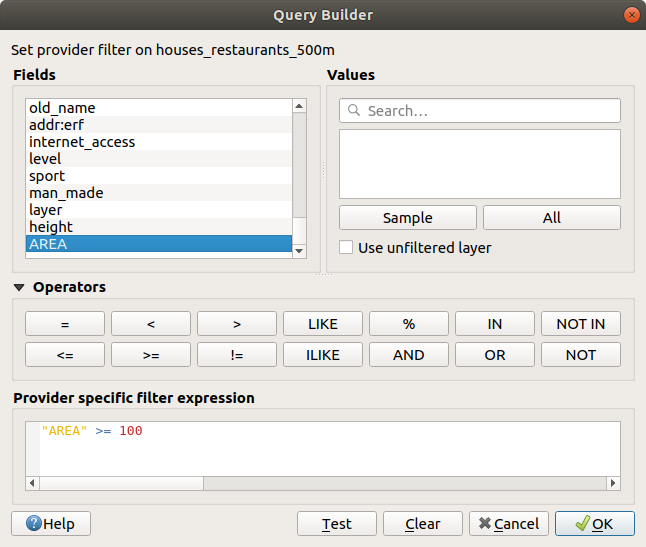
Haz clic en Aceptar.
Seu mapa agora deve mostrar apenas os edifícios que correspondem aos nossos critérios iniciais e que têm mais de 100 metros quadrados de tamanho.
6.2.12. ★☆☆ Try Yourself:
Salve sua solução como uma nova camada, usando a abordagem que você aprendeu acima para fazer isso. O arquivo deve ser salvo dentro do mesmo banco de dados GeoPackage, com o nome solução.
6.2.13. In Conclusion
Usando a abordagem de solução de problemas GIS junto com as ferramentas de análise vetorial do QGIS, você conseguiu resolver um problema com vários critérios de maneira rápida e fácil.
6.2.14. What’s Next?
Na próxima lição, veremos como calcular a distância mais curta ao longo das estradas de um ponto a outro.