중요
번역은 여러분이 참여할 수 있는 커뮤니티 활동입니다. 이 페이지는 현재 92.96% 번역되었습니다.
14.5. 수업: 체계적인 표본 설계
여러분은 이미 삼림의 수종경계를 나타내는 폴리곤 3개를 디지타이즈했지만 아직 삼림에 대한 정보를 가지고 있지는 않습니다. 이를 위해 여러분은 전체 삼림 지역의 현황 정보를 얻기 위한 조사 방법을 설계한 다음 그 파라미터를 산정할 수 있습니다. 이번 수업에서 여러분은 체계적인 표본 조사구(sampling plot) 집합을 만들 것입니다.
삼림 현황 조사를 시작했을 때 그 목적, 사용될 표본 조사구의 유형 그리고 목적을 달성하기 위해 수집될 데이터를 명확히 정의하는 것이 중요합니다. 이러한 것들은 각각의 사례에서 삼림의 유형과 관리 목적에 따라 달라지며, 삼림 관리의 지식을 가진 전문가가 신중히 계획해야 합니다. 이번 수업에서 여러분은 체계적인 표본 조사구 설계에 기초한 이론적인 현황 조사를 시행하게 될 것입니다.
이 수업의 목표: 삼림 지역을 조사하기 위한 체계적인 표본 조사구 설계하기.
14.5.1. 삼림 현황 조사하기
삼림 현황을 조사하기 위한 여러 방법들이 있습니다. 각각 다른 목적과 상태에 적합한 방법들입니다. 예를 들어, (수종만을 고려할 경우) 삼림 현황을 조사하는 아주 정확한 방법 가운데 하나는 삼림에 직접 들어가서 모든 나무의 수종과 그 특성을 조사하는 것입니다. 이것은 면적이 작은 지역이나 특별한 상황을 제외하면 일반적으로 적용할 수 있는 방법이 아니라는 것을 쉽게 알 수 있겠죠.
삼림의 정보를 알아내는 가장 일반적인 방법은 삼림 곳곳에서 측정한 표본을 만들어 전체 삼림으로 정보를 일반화하는 것입니다. 대부분의 경우 이러한 측정은 손쉽게 측정할 수 있는 작은 삼림 지역인 표본 조사구 에서 이뤄집니다. 표본 조사구는 어떤 크기(예를 들어 50 제곱미터, 0.5 헥타르 등)도 될 수 있고 어떤 형태(다양한 크기의 원형, 사각형 등)도 될 수 있으며, 그 위치도 다양한 방법(임의적, 체계적, 선형 등)으로 선정할 수 있습니다. 표본 조사구의 크기, 형태 그리고 위치는 일반적으로 통계적, 경제적 그리고 실질적인 사항을 고려하여 결정됩니다. 만약 여러분들이 삼림관리에 대한 지식이 없다면 이 위키피디아 내용 을 읽어보시기 바랍니다.
14.5.2. ★☆☆ 따라해보세요: 체계적 표본 조사구 설계 구현하기
여러분이 작업할 삼림에서, 관리자가 이 삼림에 체계적인 표본 설계가 가장 적절하다고 결정했고, 직선을 따라 80m 간격으로 표본을 선정하는 방법이 신뢰할 수 있는 결과(이 경우 68%의 신뢰도에서 표준오차 ±5%)를 얻을 수 있다고 생각합니다. 이 수목의 생장 및 성숙 수종경계 목록화 작업에 가장 효율적인 방법은 다양한 크기의 조사구를 선정하는 것이지만, 묘목 수종경계에 대해서는 4m 반경의 조사구를 이용할 것입니다.
실습 시 여러분은 표본 조사구를 단순히 포인트로 표현하면 되는데, 나중에 현장 조사팀이 이 포인트들을 사용할 것입니다.
이전 수업에서 저장했던
digitizing_2012.qgs프로젝트를 여십시오.Remove all the layers except
forest_stands_2012.이제 프로젝트를
forest_inventory.qgs라는 이름으로 저장하십시오.
지금부터 포인트 사이의 간격이 80m인 정사각형 포인트 그리드를 만들어야 합니다.
 Regular points 메뉴 항목을 클릭하십시오.
Press the drop-down button next to the Input extent field and from the Calculate from Layer menu, select
forest_stands_2012.Point spacing/count 설정에
80 meters라고 입력하십시오.이 값이 포인트들 사이의 거리를 의미하도록 Use point spacing 체크박스를 체크하십시오.
Regular points 아래에, 산출물의 경로를
forestry\sampling\폴더로 그리고 이름을systematic_plots.shp로 저장하십시오.Open output file afer running algorithm 옵션을 체크하십시오.
Run 을 클릭합니다.
참고
제안한 Regular points 도구가 선택한 폴리곤 레이어의 범위의 좌상단 모서리에서 시작하는 체계적인 포인트들을 생성합니다. 이 정규 포인트들에 어떤 임의성을 부여하고 싶은 경우, 도구 대화창의 Initial inset from corner (LH side) 파라미터에 0에서 80까지 (이때 80은 포인트들 사이의 거리입니다) 사이에서 랜덤하게 계산된 숫자를 입력하면 됩니다.
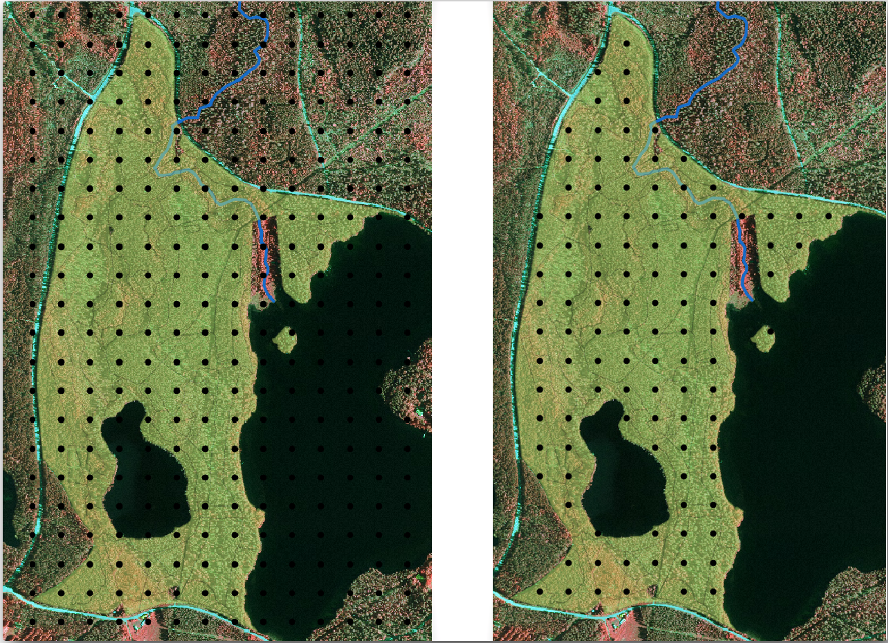
이 도구가 수종경계 레이어의 전체 범위에 정사각형 포인트 그리드를 생성했다는 것을 알 수 있습니다. 하지만 실제로는 삼림 지역 내부에 있는 포인트만 사용해야 합니다(다음 이미지들을 참조하십시오):
공간 처리 툴박스에서
 메뉴 항목을 클릭하십시오.
Select
systematic_plotsas the Input layer.Set
forest_stands_2012as the Mask layer.Clipped (mask) 결과물의 경로를
forestry\sampling\폴더로 그리고 이름을systematic_plots_clip.shp로 저장하십시오.Open output file afer running algorithm 옵션을 체크하십시오.
Run 을 클릭합니다.
이제 현장 조사팀이 지정된 표본 조사구의 위치를 찾아가는데 사용할 수 있는 포인트들을 생성했습니다. 그런데 현장 조사에 더욱 유용하도록 이 포인트들을 손볼 수 있습니다. 최소한, 포인트에 의미있는 이름을 부여해서 현장 조사팀의 GPS 기기에서 사용할 수 있는 포맷으로 내보낼 수 있을 것입니다.
표본 조사구들에 이름을 지어줍시다. 삼림 지역 안에 있는 조사구의 Attribute table 을 확인해보면 Regular points 도구가 자동 생성한 기본 id 필드가 있다는 사실을 알 수 있습니다. 포인트에 라벨을 생성해서 맵에서 ID를 볼 수 있게 하고, 이 숫자들을 표본 조사구 이름의 일부로 사용할 수 있을지 고려해보십시오:
systematic_plots_clip레이어의 Labels 메뉴를 선택하십시오.
최상단 메뉴를
Single Labels 로 전환하십시오.Value 항목에
id필드를 선택하십시오. Buffer 탭으로 가서 Draw text buffer 옵션을 체크한 다음 버퍼의 Size 를
 1로 설정하십시오.:guilabel:`OK`를 클릭하십시오.
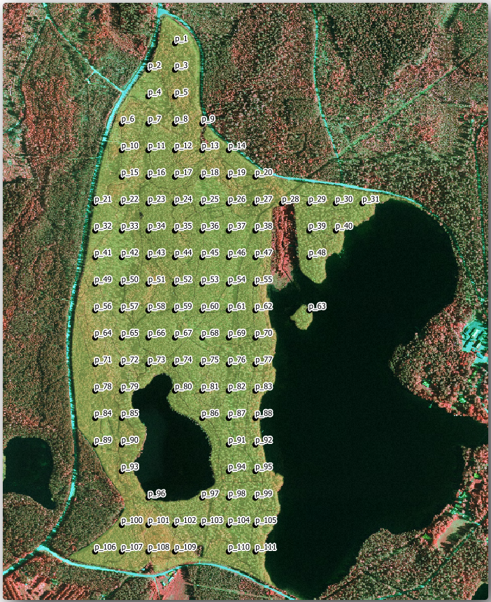
이제 맵의 라벨을 확인해보십시오. 먼저 서쪽에서 동쪽으로 그리고 북쪽에서 남쪽으로 포인트들이 생성되고 번호가 부여된 것을 볼 수 있습니다. 다시 속성 테이블을 살펴보면, 테이블 안의 포인트 순서도 이 패턴을 따른다는 사실을 알 수 있을 것입니다. 표본 조사구에 다른 방식으로 명칭을 부여할 이유가 없다면, 논리적 순서를 따라 서-동/북-남 방향으로 명명하는 것은 훌륭한 옵션이 되겠습니다.
그렇기는 하지만, id 필드의 숫자 값들이 그렇게 좋지만은 않습니다. 표본 조사구가 p_1, p_2... 같은 식의 이름이라면 더 좋겠죠. systematic_plots_clip 레이어에 새 열을 생성하면 됩니다:
systematic_plots_clip레이어의 Attribute table 을 여십시오. 편집 모드를 활성화하십시오.
 Field calculator 를 여십시오:
Create a new field 옵션을 체크하십시오.
Output field name 에
Plot_id를 입력하십시오.Output field type 을 Text (string) 으로 설정하십시오.
Expression 란에 다음
concat('P_', @row_number )공식을 입력, 복사 또는 작성하십시오. Function list 에 있는 요소들을 더블 클릭해도 된다는 사실을 기억하세요.concat함수는 String 그룹에 있고@row_number는 Variables 그룹에 있습니다.
:guilabel:`OK`를 클릭하십시오.
편집 모드를 해제하고 변경 사항을 저장하십시오.
이제 의미가 있는 조사구 이름을 가지고 있는 새 열을 만들었습니다. systematic_plots_clip 레이어에서 라벨에 쓰인 필드를 새 Plot_id 필드로 바꾸십시오.
14.5.3. ★☆☆ 따라해보세요: 표본 조사구를 GPX 포맷으로 내보내기
현장 조사팀은 아마도 여러분이 계획한 표본 조사구들의 위치를 찾아가기 위해 GPS 장치를 사용할 것입니다. 다음 단계는 여러분이 생성한 포인트들을 GPS 장치가 읽을 수 있는 포맷으로 내보내는 것입니다. QGIS는 여러분의 포인트 및 라인 벡터 데이터를 GPS 교환 포맷 (GPX) 으로 저장할 수 있게 해줍니다. GPX란 GPS 전문 소프트웨어 대부분이 읽을 수 있는 표준 GPS 데이터 포맷입니다. 데이터를 저장할 때 좌표계를 신중하게 선택해야 합니다:
systematic_plots_clip레이어를 오른쪽 클릭하면 나타나는 컨텍스트 메뉴에서 항목을 선택하십시오.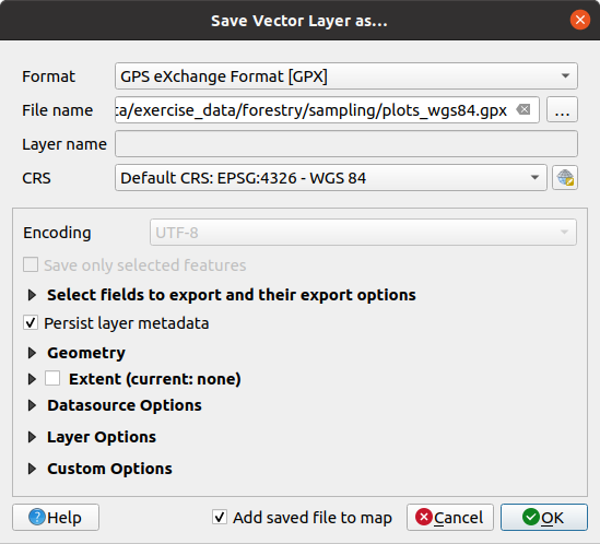
Format 에 GPS eXchange Format [GPX] 를 선택합니다.
산출물의 File name 을
forestry\sampling\경로의plots_wgs84.gpx로 저장하십시오.CRS 를 Selected CRS 로 선택합니다.
EPSG:4326 - WGS 84 를 찾으십시오.
참고
The GPX format accepts only this CRS, if you select a different one, QGIS will give no error but you will get an empty file.
:guilabel:`OK`를 클릭하십시오.
대화창이 열리면,
waypoints레이어만 선택하십시오. (나머지 레이어들은 비어 있습니다.)
현황 표본 조사구가 이제 GPS 소프트웨어 대부분이 관리할 수 있는 표준 포맷이 되었습니다. 현장 조사팀이 자신들의 GPS 장치에 표본 조사구 위치를 업로드할 수 있는 거죠. 이 작업은 여러분이 방금 저장한 plots_wgs84.gpx 파일과 특정 장치의 고유 소프트웨어를 사용해서 이루어집니다. 다른 선택지는 QGIS의 GPS Tools 플러그인을 사용하는 것이지만, 거의 대부분의 경우 특정 GPS 장치와 작업할 수 있도록 해당 도구를 설정해줘야 할 겁니다. 여러분이 자신만의 데이터를 작업하고 있는데 이 도구가 어떻게 작동하는지 알고 싶다면 QGIS 사용자 지침서 의 GPS 데이터 작업 에서 관련 정보를 찾아볼 수 있습니다.
이제 QGiS 프로젝트를 저장하십시오.
14.5.4. 결론
삼림 현황 조사에 쓰이는 체계적인 표본 설계를 얼마나 쉽게 생성할 수 있는지 확인했습니다. 다른 표본 설계 유형을 생성하려면, QGIS의 다른 도구들을 사용하거나, 스프레드시트를 이용하거나, 표본 조사구의 좌표를 계산하기 위한 스크립트를 사용해야 하지만, 기본적인 발상은 똑같습니다.
14.5.5. 다음은 무엇을 배우게 될까요?
다음 수업에서는 현장 조사팀이 표본 조사구를 찾는 데 사용할 상세 지도를 자동적으로 생성하기 위해 QGIS의 지도책 기능(Atlas capabilities)을 어떻게 사용하는지 배울 것입니다.