23.6. The batch processing interface
23.6.1. Introduction
All algorithms (including models) can be executed as a batch process. That is, they can be executed using not just a single set of inputs, but several of them, executing the algorithm as many times as needed. This is useful when processing large amounts of data, since it is not necessary to launch the algorithm many times from the toolbox.
To execute an algorithm as a batch process, right-click on its name in the toolbox and select the Execute as batch process option in the pop-up menu that will appear.
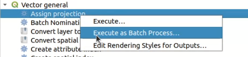
Fig. 23.31 Batch Processing from right-click
If you have the execution dialog of the algorithm open, you can also start the batch processing interface from there, clicking on the Run as batch process… button.
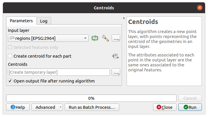
Fig. 23.32 Batch Processing From Algorithm Dialog
23.6.2. The parameters table
Executing a batch process is similar to performing a single execution of an algorithm. Parameter values have to be defined, but in this case we need not just a single value for each parameter, but a set of them instead, one for each time the algorithm has to be executed. Values are introduced using a table like the one shown next, where each row is an iteration and columns are the parameters of the algorithm.
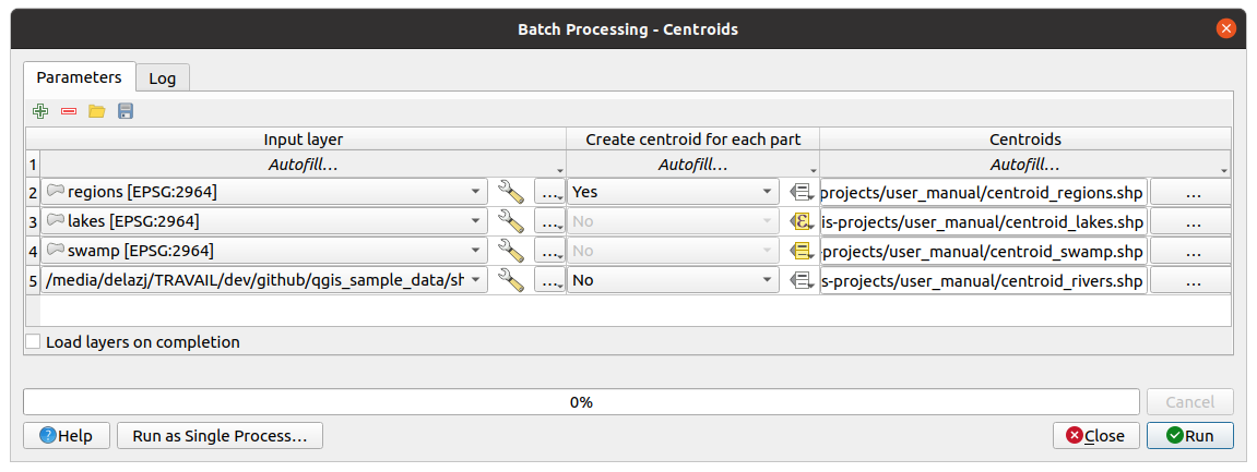
Fig. 23.33 Batch Processing
From the top toolbar, you can:
 Toggle advanced mode:
Available only when the algorithm has parameters that are marked as advanced,
this button allows to show or hide such parameters in the batch dialog.
Toggle advanced mode:
Available only when the algorithm has parameters that are marked as advanced,
this button allows to show or hide such parameters in the batch dialog. Add row: adds a new processing entry for configuration
 Remove row(s): remove selected rows from the table.
Row selection is done by clicking the number at the left and allows
keyboard combination for multi selection.
Remove row(s): remove selected rows from the table.
Row selection is done by clicking the number at the left and allows
keyboard combination for multi selection. Open a batch processing configuration file
 Save the batch processing configuration to a
 .JSONfile that can be run afterwards
By default, the table contains just two rows:
The first row displays in each cell an drop-down menu with options to quickly fill the cells below. Available options depend on the parameter type.
The second row (as well as each subsequent one) represents a single execution of the algorithm, and each cell contains the value of one of the parameters. It is similar to the parameters dialog that you see when executing an algorithm from the toolbox, but with a different arrangement.
At the bottom of the table, you can set whether to  Load
layers on completion.
Load
layers on completion.
Once the size of the table has been set, it has to be filled with the desired values.
23.6.3. Filling the parameters table
For most parameters, setting the value is trivial. The appropriate widget, same as in the single process dialog, is provided, allowing to just type the value, or select it from a list of possible values, depending on the parameter type. This also includes data-define widget, when compatible.
To automate the batch process definition and avoid filling the table cell by cell, you may want to press down the Autofill… menu of a parameter and select any of the following options to replace values in the column:
Fill Down will take the input for the first process and enter it for all other processes.
 Calculate by Expression… will allow you
to create a new QGIS expression to use to update all existing values within
that column. Existing parameter values (including those from other columns)
are available for use inside the expression via variables.
E.g. setting the number of segments based on the buffer distance of each layer:
Calculate by Expression… will allow you
to create a new QGIS expression to use to update all existing values within
that column. Existing parameter values (including those from other columns)
are available for use inside the expression via variables.
E.g. setting the number of segments based on the buffer distance of each layer:CASE WHEN @DISTANCE > 20 THEN 12 ELSE 8 END
Add Values by Expression… will add new rows using the values from an expression which returns an array (as opposed to Calculate by Expression…, which works only on existing rows). The intended use case is to allow populating the batch dialog using complex numeric series. For example adding rows for a batch buffer using the expression
generate_series(100, 1000, 50)for distance parameter results in new rows with values 100, 150, 200, …. 1000.When setting a file or layer parameter, more options are provided:
Add Files by Pattern…: adds new rows to the table for files matching a File pattern in a folder to Look in. E.g.
*.shpwill add to the list all theSHPfiles in the folder. Check Search recursively to also browse sub-folders.Select Files… individually on disk
Add All Files from a Directory…
Select from Open Layers… in the active project
Output data parameter exposes the same capabilities as when executing the algorithm as a single process. Depending on the algorithm, the output can be:
skipped, if the cell is left empty
saved as a temporary layer: fill the cell with your chosen output name, select
Create Temporary Layer from the … drop-down, and remember
to tick the Load layers on completion checkbox.
For temporary layers, the value you provide will be used as the layer name.
You can use the Autofill options to construct that name.saved as a plain file (
.SHP,.GPKG,.XML,.PDF,.JPG,…): choose Select File/Folder… from the … drop-down. For plain files, you can set the path using the Autofill options exposed beforehand.E.g. use Calculate by Expression… to set output file names to complex expressions like:
'/home/me/stuff/buffer_' || left(@INPUT, 30) || '_' || @DISTANCE || '.shp'
You can also type the file path directly or use the file chooser dialog that appears when clicking on the accompanying Select File/Folder… button. Once you select the file, a new dialog is shown to allow for auto-completion of other cells in the same column (same parameter).
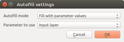
Fig. 23.34 Batch Processing Save
If the default value (Do not autofill) is selected, it will just put the selected filename in the selected cell from the parameters table. If any of the other options is selected, all the cells below the selected one will be automatically filled based on a defined criteria:
Fill with numbers: incrementally appends a number to the file name
Fill with parameter values: you can select a parameter whose value in the same row is appended to the file name. This is particularly useful for naming output data objects according to input ones.
saved as a layer within a database container:
# Indicate a layer within a GeoPackage file
ogr:dbname='C:/Path/To/Geopackage.gpkg' table="New_Table" (geom)

# Use the "Calculate By Expression" to output to different layers in a GeoPackage
'ogr:dbname=\'' || @project_folder || '/Buffers.gpkg\' table="' || @INPUT || '_' || @DISTANCE || '" (geom)'
23.6.4. Executing the batch process
To execute the batch process once you have introduced all the necessary values, just click on Run. The Log panel is activated and displays details and steps of the execution process. Progress of the global batch task will be shown in the progress bar in the lower part of the dialog.