대화창 하단에 있는 Style 메뉴를 통해 여러 대상(파일, 클립보드, 데이터베이스 등)에서/으로 이런 전체 또는 일부 속성들을 가져오거나 내보낼 수 있습니다. 사용자 지정 스타일 관리하기 를 참조하세요.
참고
원본 프로젝트 파일에서 삽입 레이어(외부 프로젝트로부터 레이어를 내포시키기 참조)의 속성들(심볼, 라벨, 액션, 기본값, 양식 등등)을 읽어오기 때문에, 이 습성을 방해할 수도 있는 변경 사항이 적용되는 일을 피하기 위해 삽입 레이어에 대해 레이어 속성 대화창을 사용할 수 없게 돼 있습니다.
Information 탭은 읽기 전용으로, 현재 레이어에 대한 요약 정보 및 메타데이터를 한 눈에 볼 수 있는 흥미로운 장소입니다. 다음과 같은 정보를 제공합니다:
프로젝트 이름, 소스 경로, 보조 파일 목록, 최신 저장 시간 및 용량, 사용하는 제공자 등의 일반 정보
custom properties, used to store in the active project additional information about the layer.
Default custom properties may include layer notes,
legend widgets, layer variables,
form properties…
More custom properties can be created and managed using PyQGIS,
specifically through the setCustomProperty() method.
레이어의 할당 좌표계 를 표시합니다. 드롭다운 목록에서 최근 사용한 좌표계를 선택하거나 Select CRS 버튼을 (좌표계 선택기 참조) 클릭해서 레이어 좌표계를 변경할 수 있습니다. 레이어에 적용된 좌표계가 틀렸거나 또는 적용된 좌표계가 없는 경우에만 변경하십시오. 사용자 데이터를 다른 좌표계로 재투영하고 싶은 경우, 공간 처리 재투영 알고리즘을 이용하거나 새 레이어로 저장 하는 편이 좋습니다.
Depending on the data provider, a Layer source group indicates the path
to the source of the dataset and allows for replacing the loaded layer:
When the layer is stored as file on disk, edit the path shown in the text box
or press …Browse to select another file on the disk.
Both layers do not need to share attribute fields, geometry type or file formats.
When the layer is provided by an ArcGIS Feature service,
it is possible to modify its authentication settings,
while keeping unchanged the details for connecting to the service.
Create spatial index (only for OGR-supported formats): helps speeding
layer rendering and features’ geometry retrieval.
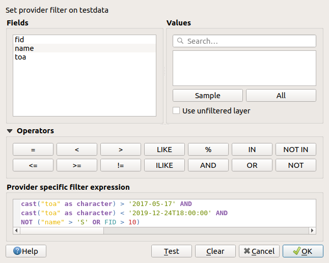
Layer 메뉴 또는 레이어의 컨텍스트 메뉴에서 Filter… 옵션을 이용해서도 Query Builder 대화창을 열 수 있습니다. 대화창의 Fields, Values 및 Operators 부분에서 Provider specific filter expression 상자에 노출되는 SQL 호환 쿼리를 작성할 수 있습니다.
필드 목록은 레이어의 모든 필드를 담고 있습니다. SQL WHERE 절 란에 속성 열을 추가하려면, 필드 목록에 있는 이름을 더블 클릭하거나 SQL 란에 직접 입력하십시오.
값 프레임은 현재 선택한 필드의 값들을 목록화합니다. 필드의 모든 유일 값들을 표시하려면, All 버튼을 클릭하십시오. 열의 처음 유일한 값 25개만 표시하려면, Sample 버튼을 클릭하십시오. SQL WHERE 절 란에 값을 추가하려면, 값 목록에 있는 이름을 더블 클릭하십시오. 값 프레임 상단에 있는 검색란을 사용하면 목록에 있는 속성 값을 쉽게 탐색하고 찾을 수 있습니다.
연산자 부분은 사용할 수 있는 모든 연산자를 담고 있습니다. SQL WHERE 절 란에 연산자를 추가하려면, 적절한 버튼을 클릭하십시오. 관계 연산자(=, > 등등), 문자열 비교 연산자(LIKE), 그리고 논리 연산자(AND, OR 등등)를 사용할 수 있습니다.
Test 버튼은 사용자의 쿼리를 점검하고 현재 쿼리를 만족하는 피처의 개수를 보여주는 메시지 창을 엽니다. Clear 버튼을 누르면 SQL 쿼리를 모두 삭제하고 레이어를 원래 상태로 (예를 들면 모든 피처를 다시 불러와) 되돌립니다. 쿼리를 .QQF 파일로 저장 Save… 할 수도 있고, 파일에서 쿼리를 대화창으로 불러올 Load… 수도 있습니다.
필터를 적용하면, QGIS는 쿼리로 선택된 하위 집합이 마치 완전한 레이어인 것처럼 취급합니다. 예를 들면, 사용자가 앞의 그림처럼 ‘Borough’ 에 대해 필터를 적용한 경우 ("TYPE_2"='Borough') Anchorage 를 표시하거나 쿼리하거나 저장하거나 편집할 수 없습니다. Anchorage 는 ‘Municipality’ 이기 때문에 하위 집합에 속하지 않기 때문입니다.
팁
레이어 패널은 필터링된 레이어를 표시합니다
Layers 패널에서 필터링된 레이어에 마우스를 가져가면 레이어 옆에 쿼리가 사용됐다는 사실을 알려주는 Filter 아이콘이 나타납니다. 이 아이콘을 더블 클릭하면 Query Builder 대화창이 열려 쿼리를 편집할 수 있습니다. 쿼리 작성기 대화창은 Layer ► Filter… 메뉴를 통해서 열 수도 있습니다.
Symbology 탭은 사용자 벡터 데이터를 렌더링하고 심볼 작업을 하기 위한 종합 도구를 제공합니다. 모든 벡터 데이터에 공통적으로 쓰이는 도구는 물론 서로 다른 벡터 데이터 유형에 맞춰 특화된 심볼 작업 도구도 이용할 수 있습니다. 하지만 모든 데이터 유형이 다음과 같은 대화창 구조를 공유합니다: 상단에는 범주화 및 피처에 적용할 심볼을 준비하는 데 쓰이는 위젯이, 하단에는 레이어 렌더링 위젯이 있습니다.
팁
서로 다른 레이어 스타일로 재빨리 바꾸기
Layer Properties 대화창 하단에 있는 Styles ► Add 메뉴를 이용하면, 스타일을 원하는 대로 얼마든지 저장할 수 있습니다. 스타일이란 레이어의 모든 (심볼, 라벨, 도표, 필드 양식, 액션 등등) 속성을 사용자가 원하는대로 조합한 것입니다. 그리고 나서, Layers Panel 에 있는 레이어의 컨텍스트 메뉴에서 스타일을 바꾸기만 하면, 사용자 데이터의 모습이 자동적으로 변경될 겁니다.
팁
벡터 심볼 내보내기
QGIS 벡터 심볼을 구글 *.kml, *.dxf 및 MapInfo *.tab 파일로 내보낼 수 있는 옵션이 존재합니다. 레이어를 오른쪽 클릭해서 컨텍스트 메뉴를 열어, Save As… 를 선택하고 산출물 파일명 및 포맷을 지정하면 됩니다. 대화창에서는 Symbology export 메뉴의 Feature symbology ► 또는 Symbol layer symbology ► 메뉴 옵션을 통해 심볼을 저장하십시오. 심볼 레이어를 사용해본 경험이 있다면, 두 번째 방법을 이용하는 편이 좋습니다.
렌더링 작업자(renderer)는 정확한 심볼과 함께 피처를 그리는 일을 책임집니다. 레이어 도형 유형에 상관없이, 렌더링 작업자에는 단일 심볼, 범주, 등급, 규칙 기반이라는 공통 유형이 4개 있습니다. 포인트 레이어의 경우, 포인트 변위(displacement), 포인트 군집 및 열지도 렌더링 작업자를 이용할 수 있는 반면 폴리곤 레이어의 경우 그 외에도 병합된 피처, 역(inverted) 폴리곤 및 2.5차원 렌더링 작업자를 통해 렌더링할 수도 있습니다.
연속 색상 렌더링 작업자라는 건 없습니다. 연속 색상 렌더링 작업자란 사실 등급 렌더링 작업자의 특수한 경우일 뿐이기 때문입니다. 심볼 및 색상표를 지정하면 심볼 색상을 적절하게 설정하는 범주 및 등급 렌더링 작업자를 생성할 수 있습니다. 각 데이터 유형(포인트, 라인 및 폴리곤) 별로, 해당 벡터 심볼 레이어 유형이 존재합니다. 어떤 렌더링 작업자를 선택하느냐에 따라, 대화창에 서로 다른 부분들이 추가될 것입니다.
참고
벡터 레이어의 스타일을 설정할 때 렌더링 작업자 유형을 변경해도, 심볼에 대한 사용자 설정은 유지될 것입니다. 다만 단 한 번 변경하는 경우에만 유지된다는 점을 기억해주십시오. 렌더링 작업자 유형을 계속 변경하다보면 심볼 설정이 사라지게 됩니다.
범주화의 Value 를 선택하십시오: 이 값은 기존 필드일 수도 있고, 사용자가 입력란에 입력하거나 또는 관련 버튼으로 작성할 수 있는 표현식 일 수도 있습니다. (예를 들어 사용자의 범주화 기준이 하나 이상의 속성으로부터 파생되는 경우) 범주화 작업에 표현식을 이용하면 심볼 범주화만을 위한 필드를 생성하지 않아도 됩니다.
피처 범주화를 위해 사용되는 표현식은 어떤 종류든 가능합니다. 예를 들어:
비교 표현식이 될 수 있습니다. 이 경우, QGIS는 1 (True)이나 0 (False)을 반환합니다. 다음은 그 예시입니다:
Indicate the Color ramp, i.e. the range of colors from which
the color applied to each symbol is selected.
색상표 위젯 의 공통 옵션 외에, 범주에 Random Color Ramp 임의의 색상표를 적용할 수 있습니다. 사용자가 만족하지 못 하는 경우 Shuffle Random Colors 를 클릭하면 새로운 임의의 색상 집합을 재생성할 수 있습니다.
그리고 Classify 버튼을 클릭해서 주어진 필드나 표현식의 개별 값으로부터 범주들을 생성하십시오.
For each class, you can edit the Legend column
to a more meaningful label (used in the Layers panel and the print layout).
참고
Keep in mind that some values may use widgets that
do not display the actual value stored in the field.
For example, a checkbox widget may store 1 and 0 for checked and unchecked
states, while displaying True and False labels. In this case,
to categorize features based on the checkbox state, you need to use
the stored values (1 and 0) in the expression.
QGIS will automatically use the display value for the legend column.
실시간 업데이트 를 사용하는 중이 아니며 맵 캔버스 상의 각 피처를 각 피처의 범주 심볼로 렌더링할 예정인 경우 Apply 를 눌러 변경 사항을 적용하십시오.
QGIS는 기본적으로 목록에 all other values 범주를 추가합니다. 처음 시작 시에는 비어 있지만, 이 범주는 다른 범주에 들어가지 않는 모든 피처를 위한 기본 범주입니다. (예를 들어 범주화 필드/표현식을 위한 새 값을 가진 피처를 생성하는 경우처럼 말이죠.)
기본 범주를 심도 있게 미세 조정할 수 있습니다:
You can Add new categories, Remove
selected categories, Delete All of them or Delete Unused categories.
범주명 왼쪽에 있는 체크박스를 해제하면 각 범주를 비활성화시킬 수 있습니다. 대응하는 피처는 맵 상에서 숨겨집니다.
드래그&드롭으로 범주의 순서를 조정할 수 있습니다.
범주의 심볼, 값 또는 범례를 변경하려면, 해당 범주를 더블 클릭하면 됩니다.
선택한 항목(들)을 오른쪽 클릭하면 나오는 컨텍스트 메뉴에는:
Copy Symbol 및 Paste Symbol: 항목의 모습을 다른 항목에 적용할 수 있는 편리한 방법입니다.
Change Color…: 선택한 심볼(들)의 색상을 변경합니다.
Change Opacity…: 선택한 심볼(들)의 투명도를 변경합니다.
Change Output Unit…: 선택한 심볼(들)의 산출물 단위를 변경합니다.
Change Width…: 선택한 라인 심볼(들)의 폭을 변경합니다.
Change Size…: 선택한 폴리곤 심볼(들)의 크기를 변경합니다.
Change Angle…: 선택한 폴리곤 심볼(들)의 기울기를 변경합니다.
Merge Categories: 선택한 여러 범주들을 단일 그룹으로 병합합니다. 이렇게 하면 수많은 범주들을 가진 레이어들의 스타일 작업을 좀 더 단순하게 할 수 있습니다. 수많은 개별 범주들을 더 적고 더 관리하기 쉬운 범주 집합으로 그룹화해서 여러 값들에 적용시키는 것도 가능할 것입니다.
팁
목록에서 선택한 범주 가운데 가장 위에 있는 심볼이 병합된 범주들 용으로 쓰일 심볼이기 때문에, 병합 전에 사용자가 재사용하고자 하는 심볼을 가진 범주를 제일 위로 이동시키는 편이 좋습니다.
Unmerge Categories: 이전에 병합한 범주들을 다시 개별 범주들로 분리합니다.
생성된 범주들은 Layers 패널에 있는 트리 위계에도 나타납니다. 레이어 패널에서 항목을 하나 더블클릭하면 할당된 심볼을 편집할 수 있습니다. 항목을 오른쪽 클릭하면 더 많은 옵션 에 접근할 수 있습니다.
Advanced 메뉴는 범주화 작업의 속도를 향상시키거나 심볼 렌더링을 미세 조정할 수 있는 옵션을 제공합니다:
Match to saved symbols: 각 범주에 범주의 범주화 값을 나타내는 이름을 가진 심볼을 심볼 라이브러리 를 사용해서 할당합니다.
Match to symbols from file…: 심볼을 보유한 파일을 지정해서, 각 범주에 범주의 범주화 값을 나타내는 이름을 가진 심볼을 할당합니다.
Graduated 렌더링 작업자는 선택한 피처의 속성이 어떤 범주에 할당되는지를 반영하는 사용자 지정 심볼의 색상 또는 크기를 이용해서 레이어의 모든 피처를 렌더링합니다.
범주 렌더링 작업자처럼, 등급 렌더링 작업자는 지정한 열로부터 심볼의 기울기 및 크기 척도를 설정할 수 있습니다.
또한 범주 렌더링 작업자처럼, 다음 옵션들을 설정할 수 있습니다:
범주화의 Value: 이 값은 기존 필드일 수도 있고, 사용자가 입력란에 입력하거나 또는 관련 버튼으로 작성할 수 있는 표현식 일 수도 있습니다. (예를 들어 사용자의 범주화 기준이 하나 이상의 속성으로부터 파생되는 경우) 범주화 작업에 표현식을 이용하면 심볼 범주화만을 위한 필드를 생성하지 않아도 됩니다.
그 다음 할당된 필드 또는 표현식에서 나온 값의 대화형 히스토그램을 표시하는 히스토그램 탭을 이용할 수 있습니다. 히스토그램 위젯을 통해 범주 단계(class break)를 이동하거나 추가할 수 있습니다.
참고
통계 요약 패널을 통해 사용자 벡터 레이어에 관한 정보를 더 많이 얻을 수 있습니다. 통계 요약 패널 을 참조하세요.
범주 탭으로 돌아가면, 범주의 개수는 물론 각 범주에 있는 범주화 기능 모드도 (모드 목록을 이용해서) 설정할 수 있습니다. 다음 모드들을 선택할 수 있습니다:
동일 개수(Equal Count; Quantile): 각 범주가 동일한 개수의 요소를 가지게 됩니다. (상자 수염 그림 개념입니다.)
동일 간격(Equal Interval): 각 범주가 동일한 크기를 가지게 됩니다. (예를 들어 1에서 16까지의 값을 범주 4개로 설정하면, 각 범주의 크기는 4가 됩니다.)
고정 간격(Fixed Interval): 각 범주가 고정된 값의 범위를 가지게 됩니다. (예를 들어 1에서 16까지의 값을 간격 크기 4로 설정하면, 범주들이 1-4, 5-8, 9-12 그리고 13-16이 됩니다.)
대수 척도(Logarithmic Scale): 값이 광범위한 데이터에 적합합니다. 적은 값에는 촘촘한 범주를, 큰 값에는 넓은 범주를 할당합니다. (예를 들어 [0..100] 범위의 십진수를 범주 2개로 설정하면, 처음 범주는 0에서 10까지, 다음 범주는 10에서 100까지가 될 것입니다.)
Natural Breaks (Jenks): 각 범주 내부의 분산량은 최소화되는 반면 범주 간의 분산량은 최대화되는 모드입니다.
Pretty Breaks: x값의 범위를 커버하면서 동일한 간격으로 보기 좋게 분포된 n+1개의 일련의 값들을 계산합니다. 10의 거듭제곱을 1, 2 또는 5로 곱한 수를 값으로 선택합니다. (R 통계 환경의 pretty 에 기반한 모드입니다.)
표준 편차: 값들의 표준 편차에 따라 범주를 생성합니다.
Symbology 탭의 가운데에 있는 목록 상자는 범주가 렌더링될 범위, 라벨, 심볼을 포함하는 범주 목록을 담고 있습니다.
Classify 버튼을 클릭해서 선택한 모드를 통해 범주를 생성하십시오. 범주명 왼쪽에 있는 체크박스를 해제하면 각 범주를 비활성화시킬 수 있습니다.
범주의 심볼, 값 그리고/또는 라벨을 변경하려면, 그냥 사용자가 원하는 항목을 더블 클릭하면 됩니다.
선택한 항목(들)을 오른쪽 클릭하면 나오는 컨텍스트 메뉴에는:
Copy Symbol 및 Paste Symbol: 항목의 모습을 다른 항목에 적용할 수 있는 편리한 방법입니다.
Change Color…: 선택한 심볼(들)의 색상을 변경합니다.
Change Opacity…: 선택한 심볼(들)의 투명도를 변경합니다.
Change Output Unit…: 선택한 심볼(들)의 산출물 단위를 변경합니다.
Change Width…: 선택한 라인 심볼(들)의 폭을 변경합니다.
Change Size…: 선택한 폴리곤 심볼(들)의 크기를 변경합니다.
Change Angle…: 선택한 폴리곤 심볼(들)의 기울기를 변경합니다.
그림 12.5 는 QGIS 예시 데이터셋의 major_rivers 레이어에 대한 등급 렌더링 작업자 대화창의 예시입니다.
심볼 트리의 상단에 있는 항목을 선택한 다음, (포인트 레이어의) Size 또는 (라인 레이어의) Width 옵션 옆에 있는 Data-defined override버튼 을 클릭하십시오.
필드를 선택하거나 표현식을 입력하면, QGIS가 각 피처별로 속성에 산출 값을 적용하고 맵 캔버스에 있는 심볼의 크기를 비례에 맞춰 재조정할 것입니다.
필요하다면 메뉴의 Size assistant… 옵션을 사용해서 심볼 크기 재조정에 몇몇 (지수, 플래너리 등등) 변환을 적용하십시오. (자세한 내용은 데이터 정의 어시스턴트 인터페이스 사용하기 를 참조하세요.)
레이어 패널 과 인쇄 조판기 범례 항목 에 비례 심볼을 표시하도록 선택할 수 있습니다: Symbology 탭의 주 대화창 하단에 있는 Advanced 드롭다운 목록을 펼치고 Data-defined size legend… 를 선택하면 범례 항목을 환경 설정할 수 있습니다. (자세한 내용은 데이터 정의 크기 범례 를 참조하세요.)
다변량 분석 생성하기
다변량 분석 렌더링은 2개 이상의 변수들 사이의 관계를 평가할 수 있습니다. 예를 들면 변수 하나를 크기로 표현하고, 다른 변수를 색상표로 표현할 수 있습니다.
QGIS 에서 다변량 분석을 생성하는 가장 간단한 방법은 다음과 같습니다:
먼저 모든 범주에 동일한 심볼 유형을 이용해서 레이어 상에 범주 또는 등급 렌더링을 적용하십시오.
규칙이란 피처에 특정 렌더링 설정을 적용하기 위해 피처의 속성(attribute) 또는 속성(property)에 따라 피처를 구분하는 데 쓰이는 QGIS 표현식 을 말합니다. 규칙은 내포될 수 있으며, 피처가 모든 상위 내포 수준(들)에 속하는 경우 피처는 범주에 속합니다.
따라서 Rule-based 렌더링 작업자는 선택한 피처를 세분화된 범주에 할당하는지를 반영하는 측면을 가진 심볼을 이용해서 레이어의 모든 피처를 렌더링하도록 설계되었습니다.
규칙을 생성하려면:
기존 행을 더블클릭해서 활성화시키거나 (QGIS는 기본적으로 렌더링 모드가 활성화될 때 규칙을 가지지 않은 심볼을 추가합니다) 또는 Edit rule 또는 Add rule 버튼을 클릭하십시오.
Edit Rule 대화창이 열리면 사용자가 각 규칙을 쉽게 식별하도록 해주는 라벨을 정의할 수 있습니다. Layers Panel 은 물론 인쇄 작성자 범례도 이 라벨을 표시할 것입니다.
Filter 옵션 옆에 있는 텍스트란에 표현식을 직접 입력하거나 그 옆에 있는 버튼을 클릭해서 표현식 문자열 작성자 대화창을 여십시오.
제공되는 함수들과 레이어 속성을 사용해서 사용자가 가져오고 싶은 피처를 필터링하기 위한 표현식 을 작성하십시오. 쿼리 결과를 확인하려면 Test 버튼을 클릭하십시오.
규칙을 요약한 새로운 행이 레이어 속성 대화창에 추가됩니다. 앞에서 설명한 단계를 따라 필요한 만큼 많은 규칙을 생성할 수도 있고 기존 규칙을 복사해서 붙여넣을 수도 있습니다. 규칙을 내포시키고 하위 범주에서 상위 규칙 피처들을 개선하려면 규칙을 다른 규칙 위로 드래그&드롭하십시오.
규칙 기반 렌더링 작업자를 범주 또는 등급 렌더링 작업자와 결합시킬 수 있습니다. 규칙을 하나 선택하면, Refine selected rules 드롭다운 메뉴를 이용해서 하위 범주에 해당 규칙이 적용된 피처를 정리할 수 있습니다. 세분화된 범주는 트리 계층에 규칙의 하위 항목처럼 나타나며, 상위 범주와 마찬가지로 사용자가 각 범주의 심볼과 규칙을 설정할 수 있습니다. 다음을 기반으로 규칙 세분화를 자동화할 수 있습니다:
축척(scales): 이 옵션은 축척 목록을 지정해서 서로 다른 사용자 정의 축척 범위가 적용되는 범주 집합을 생성합니다. 각각의 새로운 축척 기반 범주가 고유한 심볼과 정의(definition) 표현식을 가질 수 있습니다. 축척 기반 범주는 예를 들어 동일한 피처를 서로 다른 축척에서 서로 다른 심볼로 표시하거나, 또는 축척에 따라 특정 피처 집합만 표시하는 데 (예를 들면 대축척에서 지방 공항을 표시하고 소축척에서는 국제 공항을 표시하는 데) 편리한 방법입니다.
범주(categories): 선택한 규칙에 해당하는 피처에 범주 렌더링 작업자 를 적용합니다.
또는 범위(ranges): 선택한 규칙에 해당하는 피처에 등급 렌더링 작업자 를 적용합니다.
세분화된 범주는 트리 계층에 규칙의 하위 항목처럼 나타나며, 상위 범주와 마찬가지로 사용자가 각 범주의 심볼을 설정할 수 있습니다. 내포된 규칙의 심볼은 층층이 쌓이기 때문에 신중하게 선택하십시오. 이 층층이 쌓인 심볼 가운데 특정 심볼의 렌더링을 방지하기 위해 Edit rule 대화창에서 Symbols 를 체크 해제할 수도 있습니다.
Edit rule 대화창에서, 모든 규칙을 직접 작성하지 않고서도 동일 수준에서 어떤 규칙과도 일치하지 않는 모든 피처를 걸러내는 Else 옵션을 사용할 수 있습니다. Layer Properties ► Symbology ► Rule-based 대화창의 규칙(Rule) 열에 Else 를 입력해도 동일한 결과를 얻을 수 있습니다.
선택한 항목(들)을 오른쪽 클릭하면 나오는 컨텍스트 메뉴에는:
Copy 와 Paste: 기존 항목(들)을 기반으로 새 항목(들)을 생성할 수 있는 편리한 방법입니다.
Copy Symbol 및 Paste Symbol: 항목의 모습을 다른 항목에 적용할 수 있는 편리한 방법입니다.
Change Color…: 선택한 심볼(들)의 색상을 변경합니다.
Change Opacity…: 선택한 심볼(들)의 투명도를 변경합니다.
Change Output Unit…: 선택한 심볼(들)의 산출물 단위를 변경합니다.
Change Width…: 선택한 라인 심볼(들)의 폭을 변경합니다.
Change Size…: 선택한 폴리곤 심볼(들)의 크기를 변경합니다.
Change Angle…: 선택한 폴리곤 심볼(들)의 기울기를 변경합니다.
Refine Current Rule: 현재 규칙을 축척, 범주 또는 범위 로 미세 조정할 수 있는 하위 메뉴를 엽니다. 대화창 하단에서 대응하는 메뉴 를 선택하는 것과 동일합니다.
규칙 기반 렌더링 작업자 대화창에서 한 행을 체크 해제하면 맵 캔버스에서 특정 규칙과 내포된 규칙을 가진 피처를 숨깁니다.
생성된 규칙들은 맵 범례에 있는 트리 위계에도 나타납니다. 맵 범례에서 항목을 하나 더블클릭하면 할당된 심볼을 편집할 수 있습니다. 항목을 오른쪽 클릭하면 더 많은 옵션 에 접근할 수 있습니다.
그림 12.7 은 QGIS 예시 데이터셋의 rivers 레이어에 대한 규칙 기반 렌더링 작업자 대화창의 예시입니다.
Point Displacement 렌더링 작업자는 서로 지정한 허용 오차 거리에 들어오는 포인트 피처들을 받아서, 다양한 배치 방법에 따라 그 무게중심(barycenter) 주위에 심볼들을 배치합니다. 이 렌더링 작업자는 (예를 들어 같은 건물 안에 있는 오락시설들처럼) 포인트 레이어의 피처들이 동일한 위치에 존재하더라도 모두 가시화시킬 수 있는 편리한 방법이 될 수 있습니다.
포인트 변위 렌더링 작업자를 환경 설정하려면, 다음 작업을 해줘야 합니다:
Center symbol: 중심에 있는 가상 포인트가 어떻게 보일지를 결정하는 중심 심볼을 설정합니다.
Renderer: 레이어의 피처를 어떻게 분류할지를 결정하는 (단일, 범주, 규칙 기반 등등의) 렌더링 작업자 유형을 선택합니다.
Renderer Settings… 버튼을 눌러서 선택한 렌더링 작업자에 따라 피처의 심볼을 환경 설정하십시오.
Distance: 서로 근접한 피처들을 중첩해 있다고 간주하고 동일한 가상 포인트 주위로 이동시킬 허용 오차 거리를 설정하십시오. 흔히 쓰이는 심볼 단위들을 지원합니다.
Placement methods: 배치 방법을 환경설정합니다:
고리(Ring): 표시할 피처 개수에 따라 반경이 달라지는 원 위에 모든 피처를 배치합니다.
동심 고리(Concentric rings): 동심원 집합을 이용해서 피처를 표시합니다.
그리드(Grid): 각 교차점에 포인트 심볼을 가진 정규 그리드를 생성합니다.
이동된 심볼은 Displacement lines 상에 배치됩니다. 변위 라인(displacement line)의 최소 간격은 포인트 심볼 렌더링 작업자의 설정을 따르지만, 그래도 Stroke width, Stroke color 및 Size adjustment 와 같은 일부 설정을 사용자 지정할 수 있습니다. (예를 들어 이런 사용자 지정 설정을 통해 렌더링된 포인트 사이의 간격을 늘릴 수 있습니다.)
Labels 그룹 옵션을 이용해서 포인트 라벨 작업을 수행할 수 있습니다. 라벨은 피처의 실제 위치가 아니라 이동된 심볼 근처에 배치됩니다.
Label attribute: 라벨 작업에 사용할 레이어의 필드를 선택합니다.
Label font: 라벨 글꼴의 속성 및 크기를 설정합니다.
Label color: 색상을 선택합니다.
Label distance factor: 각 포인트 피처에 대해, 심볼 중심으로부터 심볼의 대각선 크기에 비례해서 라벨을 오프셋시킬 거리 인자를 설정합니다.
Use scale dependent labeling: 지정한 Minimum map scale 을 초과하는 축척에서만 라벨을 표시하고자 하는 경우 이 옵션을 체크하십시오.
포인트 변위 렌더링 작업자는 피처 도형을 변경하지 않습니다. 즉 포인트가 제자리를 벗어나지 않는다는 뜻입니다. 포인트들은 초기 위치에 그대로 자리합니다. 그저 렌더링 목적을 위해 시각적으로만 바뀔 뿐입니다. 변위된 피처를 생성하고자 하는 경우 포인트 변위시키기 공간 처리 알고리즘을 대신 사용하십시오.
최근접 또는 중첩 포인트 피처 배치를 과장하는 Point Displacement 렌더링 작업자와는 달리, Point Cluster 렌더링 작업자는 근접 포인트들을 단일하게 렌더링된 마커 심볼 하나로 그룹화합니다. 서로 특정 거리 안에 있는 포인트들을 단일 심볼로 병합하는 것이죠. 단순히 검색 거리 안에 있는 첫번째 그룹에 할당하기 보다는, 형성되는 그룹 가운데 가장 가까운 그룹을 기반으로 포인트 집합체를 생성합니다.
주 대화창에서 다음과 같은 작업을 할 수 있습니다:
Cluster symbol 에서 포인트 군집을 표현하기 위한 심볼을 설정할 수 있습니다. 기본 렌더링은 글꼴 마커 심볼 레이어 상의 @cluster_size변수 의 도움으로 합쳐진 피처들의 개수를 표시합니다.
Renderer: 예를 들어 레이어의 피처를 어떻게 분류할지를 결정하는 (단일, 범주, 규칙 기반 등등의) 렌더링 작업자 유형을 선택할 수 있습니다.
Renderer Settings… 버튼을 누르면 평소와 같이 피처의 심볼을 환경 설정할 수 있습니다. 이 심볼은 군집화되지 않은 피처에만 표시되며, 군집화된 피처에는 Cluster symbol 이 적용된다는 사실을 기억하십시오. 또한 군집에 있는 모든 포인트 피처가 동일한 렌더링 범주에 속해 있기 때문에 동일한 색상이 적용될 경우, 이 색상은 군집의 @cluster_color 변수를 표현합니다.
Distance: 피처들이 군집하는지 판단하는 데 고려할 최대 거리를 설정할 수 있습니다. 흔히 쓰이는 심볼 단위들을 지원합니다.
포인트 군집 렌더링 작업자는 피처 도형을 변경하지 않습니다. 즉 포인트가 제자리를 벗어나지 않는다는 뜻입니다. 포인트들은 초기 위치에 그대로 자리합니다. 그저 렌더링 목적을 위해 시각적으로만 바뀔 뿐입니다. 군집 기반 피처를 생성하고자 하는 경우 k-평균 군집 형성 또는 DBSCAN 군집 형성 공간 처리 알고리즘을 대신 사용하십시오.
With the Heatmap renderer you can create live
dynamic heatmaps for (multi)point layers.
You can specify the heatmap Radius in millimeters, points, pixels, map units or
inches, choose and edit a Color ramp for the heatmap style and use a slider for
selecting a trade-off between render speed and quality. You can also define a
Maximum value limit and Weight points by using a field or an expression.
Use Data defined override to dynamically control Radius and
Maximum value based on the attributes of your data.
For example, the radius of a heatmap point could be determined by its population attribute,
or the maximum value could be based on a temporal range.
When adding or removing a feature the heatmap renderer updates the heatmap style
automatically. The Color ramp will be shown as a legend bar and
in the Legend settings you can set the Labels for the Maximum
and Minimum values. You can also change the orientation and direction of the legend
in the Layout.
2.5D 렌더링 작업자를 이용해서 사용자 레이어의 피처에 2.5D 효과를 줄 수 있습니다. 먼저 Height 값(맵 단위)을 설정하십시오. 고정값, 사용자 레이어의 필드 가운데 하나, 또는 표현식으로 설정할 수 있습니다. 또 시각의 방향을 (0° 는 서쪽으로, 값이 올라갈수록 반시계 방향으로 돕니다) 재현하려면 Angle (도 단위)을 설정해야 합니다. Roof Color 및 Wall Color 을 설정하려면 고급 환경 설정 옵션을 사용하십시오. 만약 피처의 벽에 태양광 효과를 주고 싶다면, Shade walls based on aspect 옵션을 체크하도록 하십시오. Color 및 Size 값(맵 단위)을 설정하면 그림자 효과를 줄 수도 있습니다.
2.5D 렌더링 작업자에서 기본 스타일 설정을 마치고 나면, 다른 (단일 심볼, 범주, 등급) 렌더링 작업자로 변환시킬 수 있습니다. 2.5D 효과가 지속되는 동시에 다른 렌더링 작업자의 모든 특정 옵션도 쓸 수 있어 2.5D 효과를 정밀하게 조정할 수 있습니다. (예를 들어 멋진 2.5D 표현으로 범주 심볼을 그리거나 2.5D 심볼에 몇몇 기타 스타일을 추가할 수도 있습니다.) 그림자 및 “건물” 자체가 주변의 다른 피처를 가리지 않도록 하려면, 심볼 수준(Advanced ► Symbol levels…)을 활성화해야 할 수도 있습니다. 2.5D 높이 및 각도 값은 레이어의 변수에 저장되기 때문에, 이후 레이어 속성 대화창의 변수 탭에서 편집할 수 있습니다.
심볼 탭에서 레이어의 모든 피처에 대해 일괄적으로 적용되는 다음 옵션들을 설정할 수도 있습니다:
Opacity: 이 도구를 통해 맵 캔버스에서 아래에 있는 레이어를 가시화할 수 있습니다. 슬라이드 바를 통해 사용자 벡터 레이어의 가시성을 필요에 따라 조정하십시오. 슬라이드 바 옆에 있는 메뉴에서 가시성을 정확한 백분율로 설정할 수도 있습니다.
Blending mode at the Layer and Feature levels:
You can achieve special rendering effects with these tools that you may previously
only know from graphics programs. The pixels of your overlaying and
underlying layers are mixed through the settings described in 혼합 모드.
Control feature rendering order: 피처 속성을 이용해서 피처를 어떤 순서로 렌더링해야 하는지에 대한 Z 순서를 정의할 수 있습니다. 체크박스를 체크한 다음 옆에 있는 버튼을 클릭하십시오. Define Order 대화창이 열리는데, 다음 작업들을 할 수 있습니다:
레이어 피처에 적용시킬 필드를 선택하거나 표현식을 작성합니다.
불러온 피처들을 어떤 순서로 배열할지 설정합니다. 예를 들어 오름차순(Ascending) 을 선택했다면, 높은 값을 가진 피처 아래에 낮은 값을 가진 피처를 렌더링합니다.
NULL 값을 반환하는 피처를 언제, 즉 맨 처음 (아래) 또는 마지막 (위)으로 렌더링할지 정의합니다.
사용자가 사용하고자 하는 규칙에 따라 앞의 단계를 얼마든지 반복하십시오.
첫 번째 규칙은 레이어에 있는 모든 피처에 적용돼, 반환 값에 따라 피처들을 Z 순서로 배열합니다. 그 다음 규칙은 동일한 (NULL 값 포함) 값을 가진, 즉 동일한 Z 수준의 각 피처 그룹에 적용돼 각 그룹에 있는 항목들을 배열합니다. 그 다음 규칙은 다시…
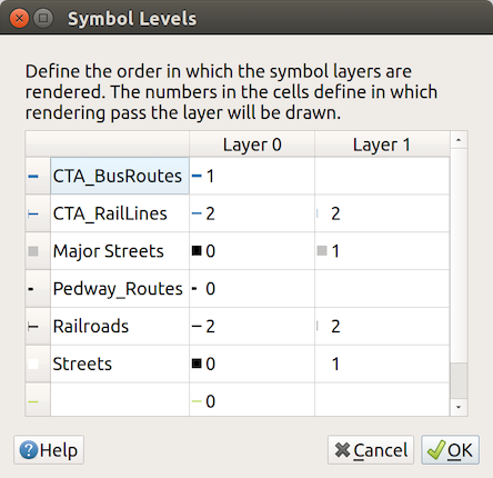
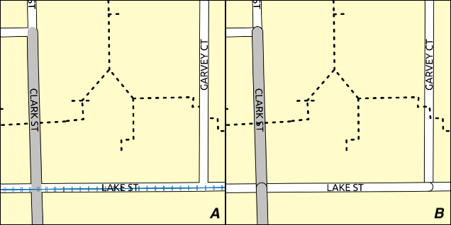
적층(積層) 심볼 레이어를 지원하는 (열지도 제외) 렌더링 작업자의 경우 각 심볼 수준의 렌더링 순서를 조정하는 옵션이 존재합니다.
대부분의 렌더링 작업자의 경우, 저장된 심볼 목록 하단에 있는 Advanced 버튼을 클릭한 다음 Symbol levels 를 선택하면 심볼 수준 옵션에 접근할 수 있습니다. 규칙 기반 렌더링 작업자 의 경우 Symbols Levels… 버튼으로 이 옵션에 직접 접근할 수 있는 반면, 포인트 변위 렌더링 작업자 의 경우 Rendering settings 대화창에 동일한 버튼이 있습니다.
심볼 수준을 활성화하려면, Enable symbol levels 를 체크하십시오. 복합 심볼, 라벨, 그리고 열로 나누어진 개별 심볼 레이어의 작은 표본이 번호와 함께 각 행에 표시됩니다. 이 번호들은 심볼 레이어를 그릴 렌더링 순서 수준을 나타냅니다. 번호 숫자가 낮을수록 먼저 그려져 아래에 남고, 높을수록 나중에 그려져 다른 레이어 위에 있게 됩니다.
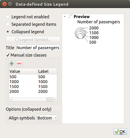
Data-defined Size Legend 대화창을 활성화시켜 심볼을 렌더링하려면, 저장된 심볼 목록 아래 있는 Advanced 버튼을 눌러 해당 옵션을 선택하십시오. 도표의 경우, Legend 탭에서 해당 옵션을 사용할 수 있습니다. 이 대화창에서 다음과 같은 옵션을 설정할 수 있습니다:
범례 유형을 선택합니다: Legend not enabled, Separated legend items 그리고 Collapsed legend 가운데 하나를 선택할 수 있습니다. 마지막 옵션을 선택했다면 범례 항목을 하단(Bottom) 정렬할지 중앙(Center) 정렬할지 선택할 수 있습니다.
사용할 범주의 크기를 재조정합니다: QGIS는 기본적으로 범례의 범주를 (Natural Pretty Breaks 기반으로) 5단계로 나눕니다. 그러나 Manual size classes 옵션을 사용하면 사용자 지정 범주를 적용시킬 수 있습니다. 및 버튼을 사용해서 사용자 지정 범주의 값과 라벨을 설정하십시오.
범례가 접혀 있는 경우:
Align symbols: 심볼을 가운데 또는 하단으로 정렬시킬 수 있습니다.
심볼에서 해당 범례 텍스트까지를 가리키는 Line symbol 수평 지시선을 환경 설정할 수 있습니다.
대화창의 오른쪽 패널에 범례의 미리보기를 표시하고, 사용자가 파라미터를 설정하는 대로 업데이트합니다.
You may set an extent buffer for a symbol. This means that a buffer is applied to
the current map extent so that if a feature is outside of the actual map extent
but inside the buffered extent it will still be rendered. This is useful for example
with symbols which use the geometry generator where you would like to still see the
generated geometries even if the actual feature is outside of the map extent.
To edit the extent buffer you can utilize the Extent buffer panel.
심볼의 최고 수준에서, 대화창 우하단에 있는 Advanced 메뉴를 선택하십시오.
Find Extent buffer option
In the new panel you can set the buffer distance
The buffer distance units can be changed. You can also control the distance value
by using the data defined override widget. For example you can change the value
based on the current map scale if(@map_scale>50000,5000,0):
그림 12.18 Example of the extent buffer with a symbol using a geometry generator symbol level.
레이어 렌더링을 향상시키고 최종 맵을 다른 소프트웨어로 렌더링하는 일을 피하기 (또는 적어도 줄이기) 위해, QGIS는 또다른 강력한 기능을 제공합니다: Draw Effects 옵션은 사용자가 벡터 레이어의 가시화를 직접 조정할 수 있도록 그리기 효과를 추가합니다.
이 옵션은 Layer Properties ► Symbology 대화창의 레이어 렌더링 그룹 (전체 레이어에 적용) 또는 심볼 레이어 속성 (해당하는 피처에 적용)에 있습니다. 이 두 옵션을 함께 사용할 수도 있습니다.
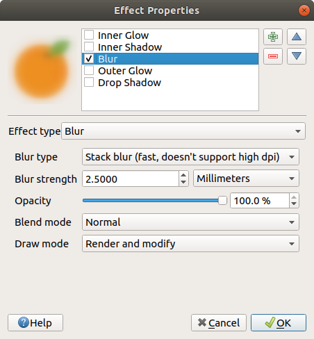
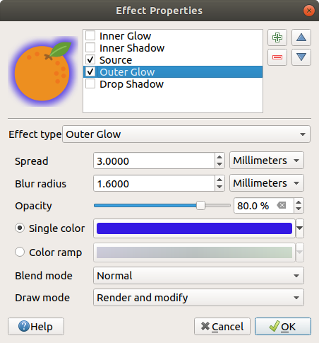
Draw effects 옵션을 체크한 다음 Customize effects 버튼을 클릭하면 그리기 효과를 활성화시킬 수 있습니다. Effect Properties 대화창이 열리는데 (그림 12.19 참조) 다음과 같은 유형의 효과들을 사용자 지정 옵션과 함께 쓸 수 있습니다:
소스(Source): 레이어 속성 환경 설정에 따라 피처의 원본 스타일을 그립니다. 해당 스타일의 혼합 모드 와 그리기 모드 는 물론, Opacity 도 조정할 수 있습니다. 이 세 가지는 모든 효과 유형의 공통 속성입니다.
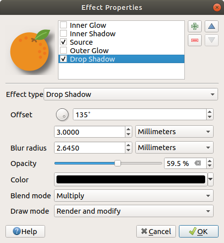
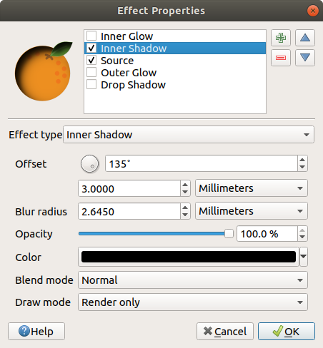
그림자 생성(Drop Shadow): 이 효과를 이용하면 객체에 그림자를 추가하는데, 마치 차원을 하나 더한 것처럼 보입니다. 그림자의 방향 및 소스 객체와의 근접도를 결정하는 Offset 각도 및 거리를 변경해서 이 효과를 사용자 지정할 수 있습니다. Drop Shadow 는 그림자 효과의 Blur radius 및 Color 를 변경할 수 있는 옵션도 보유하고 있습니다.
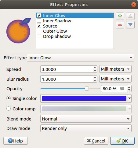
내부 광원(Inner Glow): 객체 내부에 광원 효과를 추가합니다. 광원의 Spread (너비) 또는 Blur radius 를 조정해서 이 효과를 사용자 지정할 수 있습니다. 흐리기 반경은 사용자가 흐리기 효과를 주려 하는 위치가 피처 경계선에 얼마나 근접해 있는지를 지정합니다. 또한, 광원의 색상을 Single color 또는 Color ramp 로 사용자 지정할 수 있는 옵션도 있습니다.
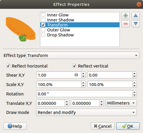
변형(Transform): 이 효과는 심볼의 형태를 변형시킬 수 있습니다. 사용자 지정을 위해 사용할 수 있는 첫 번째 옵션은 Reflect horizontal 및 Reflect vertical 으로, 수평 그리고/또는 수직 축을 기준으로 거울상을 실제로 생성합니다. 나머지 옵션 4 개는 다음과 같습니다:
Shear X,Y: X 그리고/또는 Y축을 따라 피처를 기울입니다.
Scale X,Y: X 그리고/또는 Y축을 따라 피처를 지정한 백분율로 확대하거나 축소합니다.
Rotation: 피처의 중심점을 기준으로 피처를 회전시킵니다.
Translate X,Y: X 그리고/또는 Y축을 기준으로 지정한 거리에 따라 피처의 위치를 변경합니다.
하나 이상의 그리기 효과를 동시에 줄 수 있습니다. 효과 목록에 있는 체크박스를 통해 어떤 효과를 활성화/비활성화시켜보십시오. Effect type 옵션을 이용하면 선택한 효과 유형을 변경할 수 있습니다. Move up 및 Move down 버튼으로 효과의 순서를 바꿀 수 있고, Add new effect 와 Remove effect 버튼을 통해 효과를 추가하거나 제거할 수도 있습니다.
모든 그리기 효과 유형에 사용할 수 있는 공통 옵션이 몇 개 있습니다. Opacity 및 Blend mode 옵션은 레이어 렌더링 에서 설명하는 옵션과 비슷하게 동작하며, 변형 효과를 제외한 모든 그리기 효과에 사용할 수 있습니다.
모든 그리기 효과에서 Draw mode 옵션을 쓸 수도 있는데, 심볼을 렌더링할지 그리고/또는 수정할지를 다음 몇몇 규칙에 따라 선택할 수 있습니다:
그리기 효과는 위에서 아래 순서로 렌더링합니다.
Render only 모드는 효과를 가시화할 것이라는 뜻입니다.
Modifier only 모드는 효과를 가시화하지는 않지만 적용된 변경 사항을 다음 (바로 아래에 있는) 효과로 넘길 것이라는 의미입니다.
Render and Modify 모드는 효과를 가시화하고 적용된 변경 사항을 다음 효과로 넘길 것입니다. 어떤 효과가 효과 목록 제일 위에 있거나 또는 바로 위에 있는 효과가 수정 모드가 아닌 경우, (소스 효과와 비슷하게) 레이어 속성에서 가져온 원본 소스 심볼에 해당 효과를 줄 것입니다.
Labels 속성 대화창은 벡터 레이어에 대해 스마트 라벨 작업 환경을 설정하기 위해 필요한 그리고 적절한 모든 기능을 제공합니다. Layer Styling 패널에서 또는 라벨 툴바 의 Layer Labeling Options 아이콘을 통해 이 대화창을 열 수 있습니다.
At the top of the dialog, you have:
a combobox for selecting the appropriate labeling method for the active layer
the Configure project labeling rules button:
helps you control interactions between labels and features across the layers in the project.
More details at Configuring project labeling rules.
the Automated placement settings (applies to all layers) button:
configure general properties on label placement and conflicts resolution.
More details at 자동화된 배치 엔진 설정하기.
먼저 드롭다운 목록에서 라벨 작업 방식을 선택합니다. 다음 4 개의 옵션을 사용할 수 있습니다:
대화창 상단에 Value 드롭다운 목록이 활성화됩니다. 이 목록에서 라벨 작업에 사용할 속성 열을 선택할 수 있습니다. 디스플레이 필드 를 기본값으로 사용합니다. 표현식을 바탕으로 라벨을 정의하고 싶다면 을 클릭하십시오 – 표현식을 기반으로 라벨 정의하기 를 참조하세요.
참고
범례 탭에서 라벨을 활성화시키면 범례에 라벨을 라벨 서식과 함께 항목으로 표시할 수 있습니다.
Pressing the Configure project labeling rules button
next to the labeling method drop-down selector, you can create rules
that controls how labels from a layer can interact with labels or features
from another layer.
Press the Add rule button and in the drop-down menu,
select one of the rule types:
Prevent labels overlapping features:
prevents labels being placed overlapping features from a different layer.
Pull labels towards features:
prevents labels being placed too far from features from a different layer.
The maximum distance can be set in the unit of your choice.
Push labels away from features:
prevents labels being placed too close to features from a different layer.
The minimum distance can be set in the unit of your choice,
as well as the rule’s priority
(The highest-priority rules are more important to respect
in the event of a label placement conflict).
Push labels away from other labels:
prevents labels being placed too close to labels from a different layer.
주의
The last three options are only available on QGIS installed
with GEOS >= 3.10 (see Help ► About menu).
Fill the properties at your will; you can provide a more meaningful name to the rule.
OK 를 클릭합니다.
Add as many rules as necessary.
If necessary, press Edit rule to modify the selected rule
or Remove rule to delete it from the project.
The set rules are available from any layer Labels properties tab,
pressing the Configure project labeling rules button.
You can temporary enable or disable any of them, using the checkbox next to the name.
Hover over a rule to preview its details.
자동화된 배치 설정을 사용하면 라벨의 프로젝트 수준 및 자동화된 습성 환경을 설정할 수 있습니다. Labels 탭 우상단에 있는 Automated placement settings (applies to all layers) 버튼을 클릭하면 다음 옵션을 가지고 있는 대화창이 열립니다:
Number of candidates: 라인 및 폴리곤 피처의 크기를 바탕으로 배치할 수 있는 라벨의 개수를 계산해서 피처에 할당합니다. 피처가 더 길거나 넓을수록 더 많은 후보를 가지게 되므로 해당 피처의 라벨이 충돌할 위험을 덜고 더 잘 배치할 수 있습니다.
Text rendering: sets the default value for label rendering
widgets when exporting a map canvas or
a layout to PDF or SVG.
If Always render labels as text is selected then labels can be
edited in external applications (e.g. Inkscape) as normal text. BUT the side
effect is that the rendering quality is decreased, and there are issues with
rendering when certain text settings like buffers are in place.
That’s why Always render labels as paths (recommended)
which exports labels as outlines but guarantees complete compatibility
with the full range of formatting options available, is recommended.
With Prefer rendering labels as text option, labels are rendered as text objects,
unless doing so results in rendering artifacts or poor quality rendering (depending on text format settings).
참고
When rendering labels as text to a vector based device (e.g. PDF or SVG),
care must be taken to ensure that the required fonts are available to users
when opening the created files, or default fallback fonts will be used to display the output instead.
(Although PDF exports MAY automatically embed some fonts when possible, depending on the user’s platform).
Allow truncated labels on edges of map: 일부가 맵 범위 바깥으로 벗어나는 라벨을 렌더링할지 여부를 제어합니다. 이 옵션을 체크하면 (라벨을 완전히 가시 영역 안으로 배치할 방법이 없는 경우) 이런 라벨을 표시할 것입니다. 체크를 해제하면 일부만 보이는 라벨을 무시할 것입니다. 이 설정은 조판기 맵 항목 에서의 라벨 표시에는 아무 영향도 주지 않는다는 사실을 기억하십시오.
Show all labels for all layers (i.e. including colliding objects): 이 옵션을 레이어별로 설정할 수도 있다는 사실을 기억하십시오. (렌더링 탭 참조)
Show unplaced labels: 어떤 중요한 라벨이 (예를 들면 중첩 또는 다른 제약조건 때문에) 맵에서 없어졌는지 여부를 확인할 수 있습니다. 이런 라벨은 사용자 지정 색상으로 표시됩니다.
Show candidates (for debugging): 맵 위에 라벨 배치용으로 생성된 모든 후보를 보여주는 상자들을 그릴지 여부를 제어합니다. 옵션 이름대로, 이 옵션은 디버깅 및 서로 다른 라벨 작업 설정이 주는 효과를 점검하는 데에만 유용합니다. 사용자가 직접 라벨 툴바 의 도구를 사용해서 더 나은 배치 작업을 하는 경우 이 옵션이 편리할 수도 있습니다.
Show label metrics (for debugging):
displays the text bounds of the label in red and baselines in blue
Project labeling version: QGIS는 두 가지 서로 다른 라벨 배치 자동화 버전을 지원합니다:
Version 1: (QGIS 3.10 이하 버전이 사용하는, 그리고 이전 버전에서 생성된 프로젝트 파일을 QGIS 3.12 이후 버전에서 열었을 경우 사용되는) 이전 체계입니다. 버전 1은 라벨 및 방해물의 우선 순위를 “대강의 안내” 로만 취급하기 때문에, 이 버전에서는 우선 순위가 낮은 라벨이 우선 순위가 높은 방해물 위로 배치될 수도 있습니다. 따라서 이 버전을 사용할 경우 원하는 라벨 작업 산출물을 얻기 어렵게 되므로, 옛날 프로젝트와의 호환성만을 위해 사용하는 것을 추천합니다.
Version 2 (추천): QGIS 3.12 이후 버전에서 생성된 새 프로젝트에서 사용되는 기본 체계입니다. 버전 2에서는 라벨이 방해물 을 중첩할 수 있는 경우를 규정하는 논리를 재작업했습니다. 이 새로운 논리는 어떤 라벨도 스스로의 우선 순위와 비교해 더 큰 방해물 가중치를 가진 어떤 방해물도 중첩할 수 없도록 하고 있습니다. 그 결과, 이 버전은 훨씬 예상 가능하고 쉽게 이해할 수 있는 라벨 작업 산출물을 내놓습니다.
기존 규칙들을 요약한 내용이 주 대화창에 (그림 12.31 참조) 표시됩니다. 여러 개의 규칙을 추가할 수 있고, 드래그&드롭으로 이 규칙들을 재정렬하거나 서로 겹치게 배열할 수 있습니다. 규칙을 버튼으로 제거할 수도 있고, 버튼 또는 더블클릭으로 편집할 수도 있습니다.
사용자의 라벨 속성과는 별개로 다중부분(multi-part) 피처용 라벨 작업을 설정할 수 있는 옵션이 존재합니다. 렌더링, Featureoptions 를 선택하고, Label every part of multipart-features 옆에 있는 Data-define override 버튼을 클릭한 다음 데이터 정의 무시 설정 에서 설명하는 대로 라벨을 정의하십시오.
Highlight Pinned Labels, Diagrams and Callouts: 라벨 항목이 속한 벡터 레이어가 편집 가능 상태인 경우 녹색으로 강조되고, 편집 가능 상태가 아니라면 파란색을 유지합니다.
Toggle Display of Unplaced Labels: 어떤 중요한 라벨이 (예를 들면 중첩 또는 다른 제약조건 때문에) 맵에서 누락되었는지 여부를 확인할 수 있습니다. 이런 라벨은 사용자 지정이 가능한 색상으로 표시됩니다. (자동화된 배치 엔진 설정하기 를 참조하세요.)
Pin/Unpin Labels and Diagrams. By clicking or dragging an
area, you pin overlaid items. If you click or drag an area holding Shift,
the items are unpinned. Finally, you can also click or drag an area holding
Ctrl to toggle their pin status.
Show/Hide Labels and Diagrams: 항목을 클릭하거나 kbd:Shift 키를 누른 채 어떤 영역을 클릭&드래그하면 해당 항목을 숨깁니다. 항목이 숨겨져 있는 경우, 그냥 해당 피처를 한번 클릭하면 가시성을 복원합니다. 영역을 드래그하면 해당 영역에 있는 모든 항목의 가시성을 복원할 것입니다.
Move a Label, Diagram or Callout: 항목을 클릭해서 선택한 다음 원하는 위치를 클릭해서 해당 위치로 옮깁니다. 새로운 좌표는 보조 필드 에 저장됩니다. 이 도구로 항목을 선택한 다음 Delete 키를 누르면 저장된 위치값을 삭제할 것입니다.
Rotate a Label: 라벨을 클릭해서 선택한 다음 원하는 기울기가 적용되도록 다시 클릭하십시오. 마찬가지로, 새 각도는 보조 필드에 저장됩니다. 이 도구로 라벨을 선택한 다음 Delete 키를 누르면 해당 라벨의 기울기값을 삭제할 것입니다.
Change Label Properties: 이 아이콘을 누른 다음 라벨을 클릭하면, 해당 라벨의 속성을 변경할 수 있는 대화창이 열립니다. 라벨 그 자체, 라벨의 좌표, 각도, 글꼴, 크기, 멀티라인 정렬 등등 그 속성이 필드에 매핑돼 있는 한 해당 속성을 변경할 수 있습니다. 여기에서 피처의 모든 부분에 라벨을 붙이는 Label every part of a feature 옵션을 설정할 수 있습니다.
경고
라벨 도구는 현재 필드 값을 덮어 씁니다
라벨 작업을 사용자 지정하는 데 Label toolbar 를 사용하면 매핑된 필드에 새 속성값을 실제로 작성합니다. 따라서, 사용자가 나중에 필요할 수도 있는 데이터를 무심코 덮어 쓰지 않도록 주의하십시오!
참고
기저 데이터소스를 수정하지 않은 채 라벨 작업(위치 등등)을 사용자 지정하는 데 보조 저장소 속성 메커니즘을 사용할 수도 있습니다.
Label Toolbar 와 데이터 정의 무시 설정을 결합하면 맵 캔버스에 있는 라벨을 조작할 (이동시킬, 편집할, 기울기를 적용할) 수 있습니다. 이제 Move Label, Diagram or Callout 기능에 데이터 정의 무시 기능을 이용하는 예시를 설명할 것입니다. (그림 12.35 를 참조하세요.)
QGIS 예시 데이터셋으로부터 lakes.shp 레이어를 가져옵니다.
레이어를 더블클릭해서 레이어 속성 대화창을 엽니다. Labels 탭을 선택하고 Placement 를 클릭한 다음 Offset from centroid 를 선택합니다.
Data defined 항목을 찾아 아이콘을 클릭해서 Coordinate 의 필드 유형을 정의합니다. X 값으로 xlabel 을, Y 값으로 ylabel 을 선택합니다. 이제 아이콘이 노란색으로 강조됐을 겁니다.
The Diagrams tab allows you to add a graphic overlay to
a vector layer (see 그림 12.37). This
dialog can also be accessed from the Layer Styling panel, or using
the Layer Diagram Options button of the Labels toolbar.
현재 도표의 핵심 구현은 다음을 지원하고 있습니다:
No diagrams: 기본값입니다. 피처 위로 어떤 도표도 표시하지 않습니다.
Pie chart: 원형 통계 그래픽인 원형 차트로, 숫자로 나타낸 비율을 보여주는 조각들로 나누어집니다. 각 조각의 원호 길이는 각 조각이 나타내는 양과 비례합니다.
Text diagram, a horizontally divided circle showing statistic
values inside;
Histogram, bars of varying colors for each attribute
aligned next to each other;
Stacked bars, stacks bars of varying colors for each
attribute on top of each other vertically or horizontally;
Stacked diagram, stacks diagrams of equal or varying
types, next to each other, vertically or horizontally. More details at
Stacked Diagrams.
Diagrams 탭의 우상단에 있는 Automated placement settings (applies to all layers) 버튼을 클릭하면 맵 상에 있는 도표 라벨의 배치 를 제어할 수 있습니다.
팁
도표 유형을 재빨리 바꾸기
서로 다른 도표 유형들의 설정이 거의 동일하다는 점을 고려하면, 사용자가 도표를 구성할 때 도표 유형을 쉽게 변경해서 어떤 유형이 사용자 데이터를 아무 손실 없이 적절하게 표현하는지 확인할 수 있습니다.
Rendering 탭은 도표가 어떻게 보일지를 정의합니다. 이 탭은 통계값들을 건드리지 않는, 다음과 같은 일반 설정들을 제공합니다:
그래픽의 투명도, 외곽선 너비 및 색상
도표 유형에 따라:
히스토그램과 누적 막대 그래프의 경우, 막대의 너비 및 막대 사이의 간격을 설정할 수 있습니다. 누적 막대의 경우 간격을 0 으로 설정하는 편이 좋습니다. 여기에, 라인 심볼 속성 을 사용하면 Axis line symbol 을 맵 캔버스에 보이게 하고 사용자 지정할 수 있습니다.
Diagram z-index: controls how diagrams are drawn on top of each
other and on top of labels. A diagram with a high index is drawn over other
diagrams and labels;
Show all diagrams: 서로 중첩되더라도 모든 도표를 표시합니다.
Show diagram: 특정 도표만 렌더링되도록 할 수 있습니다.
Always Show: 특정 도표가 다른 도표 또는 맵 라벨과 중첩하더라도 언제나 렌더링되도록 선택합니다.
Size 탭은 선택한 통계를 어떻게 표현할지 설정합니다. 도표의 크기 단위 는 ‘Millimeters’, ‘Points’, ‘Pixels’, ‘Map Units’ 또는 ‘Inches’ 입니다. 다음 가운데 하나를 선택할 수 있습니다:
Fixed size: 모든 피처의 그래픽을 유일한 크기로 표현합니다. (히스토그램에는 적용되지 않습니다.)
Scaled size: 레이어 속성을 이용하는 표현식을 기반으로 크기를 결정합니다:
Attribute 란에서 필드를 선택하거나 표현식을 작성한 다음
Find 를 눌러 해당 속성의 Maximum value 를 반환받거나, 위젯에 사용자 지정 값을 입력하십시오.
히스토그램과 누적 막대 그래프의 경우, 속성의 Maximum value 를 나타내는 데 사용되는 Bar length 값을 입력하십시오. 각 피처 별로 이 비율을 유지하기 위해 막대 길이를 선형적으로 축척 조정할 것입니다.
원형 차트와 텍스트 도표의 경우, 속성의 Maximum value 를 나타내는 데 사용되는 Size 값을 입력하십시오. 각 피처 별로 이 비율을 (0 에서부터) 유지하기 위해 원의 면적 또는 지름을 선형적으로 축척 조정할 것입니다. 하지만 작은 도표의 경우 Minimum size 를 설정할 수 있습니다.
Placement 탭에서 도표의 위치를 정의합니다. 레이어 도형 유형에 따라, 배치를 위한 서로 다른 옵션을 제공하고 있습니다(자세한 내용은 배치 참조):
Around point 또는 Over point: 포인트 도형 용입니다. 전자는 적용할 반경도 설정해야 합니다.
Around line 또는 Over line: 라인 도형 용입니다. 포인트 객체와 마찬가지로, 전자는 어느 한 쪽으로의 거리를 설정해야 합니다. 사용자는 객체를 기준으로 (라인의 ‘above’, ‘on’ 그리고/또는 ‘below’) 도표 배치를 지정할 수 있습니다. 한 번에 여러 옵션을 함께 선택할 수도 있습니다. 이 경우, QGIS가 도표의 최적 위치를 찾을 것입니다. 라인 방향을 이용해서 도표의 위치를 설정할 수도 있다는 점을 기억하십시오.
Around centroid (설정된 Distance 에), Over centroid, Using perimeter 및 Inside polygon: 폴리곤 객체 용 옵션입니다.
Coordinate 그룹: 피처 별로 도표 배치를 직접 제어할 수 있습니다. 피처의 속성 또는 표현식을 사용해서 X 및 Y 좌표를 설정합니다. 라벨 및 도표 이동 도구를 사용해서 좌표 정보를 채울 수도 있습니다.
In the Priority section, you can define the placement priority rank
of each diagram, i.e. if there are different diagrams or labels candidates for the
same location, the item with the higher priority will be displayed and the
others could be left out.
Discourage diagrams and labels from covering features defines
features to use as obstacles, i.e. QGIS will try to not
place diagrams nor labels over these features.
The priority rank is then used to evaluate whether a diagram could be omitted
due to a greater weighted obstacle feature.
Legend 탭에서, 레이어 패널 및 인쇄 조판기 범례 의 레이어 심볼 옆에 도표 항목을 표시할지 여부를 선택할 수 있습니다:
Show legend entries for diagram attributes: 이 옵션을 체크하면 범례에 Attributes 탭에서 할당했던 Color 및 Legend 속성을 표시합니다.
그리고 도표에 척도 크기 가 사용된 경우, Legend Entries for Diagram Size… 버튼을 클릭하면 범례에 있는 도표 심볼 속성의 환경을 설정할 수 있습니다. 이 버튼은 Data-defined Size Legend 대화창을 여는데, 데이터 정의 크기 범례 에서 이 대화창의 옵션을 설명하고 있습니다.
설정을 마치면, 인쇄 조판기 범례의 레이어 심볼 옆에도 도표 범례 항목이 (색상 및 도표 크기 속성이) 표시됩니다.
Stacked diagrams allow users to create complex diagrams like population pyramids,
where two subdiagrams, namely histograms, are located side by side and displayed
horizontally.
그림 12.41 Population pyramids built for each layer feature
Multi-temporal diagrams can also be constructed as stacked diagrams. The number
of subdiagrams, as well as the spacing between them can be configured.
Moreover, subdiagrams can have different types (e.g., a pie chart alongside a
histogram) and have their own independent settings like Attributes,
Rendering, Size,
Options and Legend.
Placement settings in a stacked diagram, as well as
some visibility settings (located in the Rendering
tab), are determined by the placement and visibility settings of the first
subdiagram in the stack.
Finally, subdiagram ordering is given by the item ordering in the Stacked Diagram’s
list. The first subdiagram appears to the left in a horizontal stacked diagram,
or in the upper part of a vertical one.
Masks 탭에서 다른 모든 레이어의 심볼 레이어 또는 라벨과 중첩하는 현재 레이어 심볼을 환경 설정할 수 있습니다. 즉 중첩하는 경우 색상이 비슷해 구분하기 힘든 심볼 및 라벨의 가독성을 향상시킬 수 있다는 뜻입니다. 항목 주변에 사용자 지정한 투명 마스크를 추가해서 현재 레이어의 심볼 레이어의 일부분을 “숨깁니다”.
활성화된 레이어에 마스크를 적용하려면, 먼저 프로젝트에서 마스크 심볼 레이어 또는 마스크 라벨 을 켜야 합니다. 그 다음 Masks 탭에서 다음을 확인하십시오:
Masked symbol layers: 현재 레이어의 모든 심볼 레이어를 트리 구조로 목록화합니다. 이 목록에서 선택한 마스크 소스와 중첩하는 경우 투명하게 “누락” 시키고자 하는 심볼 레이어 항목을 선택할 수 있습니다.
Mask sources 탭: 프로젝트에 정의되어 있는 모든 마스크 라벨과 마스크 심볼 레이어들의 목록입니다. 선택한 마스크 심볼 레이어를 덮는 마스크를 생성할 항목을 선택하십시오.
3D View 탭에서 피처의 표고 및 고도와 관련된 (Altitude clamping, Altitude binding, Extrusion 또는 Height 등의) 속성은 레이어의 표고 속성 으로부터 기본값을 상속받기 때문에, Elevation 탭 안에서 설정하는 편이 좋을 것입니다.
더 나은 성능을 위해 배후에서 멀티스레드 작업을 통해 벡터 레이어의 데이터를 불러온 다음, 타일로 렌더링합니다. 이때 3D 뷰 탭의 Layer rendering 부분에서 타일의 크기를 제어할 수 있습니다.
Zoom levels count: 사분 트리(quadtree)의 깊이를 결정합니다. 예를 들면 확대/축소 수준이 1인 경우 전체 레이어를 단일 타일로 나타냅니다. 확대/축소 수준이 3이라면 지엽(leaf) 수준에서 타일이 16개가 됩니다. (모든 추가적인 확대/축소 수준은 타일 개수가 4배수가 됩니다.) 기본값은 3 이며, 최대값은 8 입니다.
Show bounding boxes of tiles: 표시되어야 할 타일이 표시되지 않는 문제가 있을 경우 특히 유용한 옵션입니다.
Fields 탭은 레이어 관련 필드에 대한 정보를 제공하며, 레이어 필드를 정리할 수 있습니다.
Toggle editing mode 버튼으로 레이어를 편집 가능 모드로 만들 수 있습니다. 레이어가 편집 가능 모드일 경우, New field 및 Delete field 버튼을 사용해서 레이어 구조를 수정할 수 있습니다.
새 필드 New field 를 생성할 때, 주석(comment) 편집을 허용하는 데이터소스에 대해서만 Comment 옵션을 사용할 수 있습니다. 또한, 지원하는 OGR 포맷(지오패키지와 ESRI 파일 지오데이터베이스)의 경우 Add Field 대화창 안에서 별명(alias)을 설정할 수도 있습니다.
The Attributes Form tab helps you set up the form to
display when creating new features, editing or querying existing one.
This affects them in both table and form views.
You can define:
the look and the behavior (label, visibility, widget, constraints…) of each field
in the current layer, the joined layers
and the relational ones;
extra HTML, QML, text widgets to enhance the form;
양식 또는 필드 위젯과 대화형 작업을 처리하기 위한 파이썬 추가 논리
대화창 우상단에서 새 피처 생성시 양식을 기본적으로 열지 여부를 설정할 수 있습니다. Settings ► Options ► Digitizing 메뉴의 Suppress attribute form pop-up after feature creation 옵션을 통해 레이어별 또는 전체 수준으로 환경 설정할 수 있습니다.
Identify Features 도구로 피처를 클릭하거나 또는 속성 테이블을 양식 뷰(form view) 모드로 바꾸는 경우, 기본적으로 QGIS는 기본 양식을 미리 정의된 위젯과 함께 표시합니다. (일반적으로 스핀박스(spinbox)와 텍스트 상자로 이루어집니다. 지정된 행에 각 필드를 위젯 옆에 있는 필드 라벨로 표현합니다.) 만약 레이어에 관계 가 설정돼 있다면, 양식의 하단에 내장된 프레임에 참조 레이어의 필드를 동일한 기본 구조대로 표시합니다.
이 렌더링은 Layer properties ► Attributes Form 탭에 있는 Attribute editor layout 설정의 기본값 Autogenerate 의 결과입니다. 이 속성은 서로 다른 세 가지 값을 선택할 수 있습니다:
Autogenerate: 양식에 대해 “1행 - 1필드” 라는 기본 구조를 유지하지만 대응하는 각 위젯을 사용자 지정할 수 있습니다.
Drag-and-dropdesigner: 위젯 사용자 지정 외에도 양식 구조를 더 복잡하게, 예를 들어 그룹 및 탭에 위젯을 내장시키도록 만들 수 있습니다.
Provideuifile: Qt 설계자 파일을 사용할 수 있게 해줍니다. 따라서 잠재적으로 더 복잡하고 완전한 기능을 가진 템플릿을 피처 양식으로 활용할 수 있습니다.
Just below the Attribute editor layout setting, a search box allows you to
filter fields, relations, containers and other available widgets.
For items that support aliases, like fields or relations, the filter targets both
names and aliases.
The Show field aliases instead of names button allows
you to toggle field aliases and field names.
When showing aliases, fields without an alias set will have their names displayed
in light gray to help identify them easily.
그림 12.46 Search fields using aliases and names in Attributes Form page
When the Autogenerate option is on, the Available widgets panel
displays lists of fields (from the current layer, the join and relation layers)
and the enabled actions that would be shown in the form.
Select a field and you can configure its appearance and behavior in the right panel:
In this editor mode, only the properties can be viewed for the actions.
Moreover, they will be displayed through an Actions drop-down menu in the feature form,
and following the Show in attribute table property in other contexts.
드래그&드롭 설계자는 그림 12.47 에서 볼 수 있는 바와 같이 (HTML/QML 위젯 또는 레이어에 정의된 액션 처럼) 특정 필드에 직접 링크되어 있지 않은 속성 필드 또는 다른 위젯을 나타내기 위한 컨테이너(탭 또는 그룹)를 몇 개 가지고 있는 양식을 생성할 수 있게 해줍니다.
Select attribute layout editor 콤보박스에서 Draganddropdesigner 를 선택하면, Available widgets 패널 옆에 있는 Form Layout 패널을 기존 필드로 채워서 활성화합니다. 선택한 필드는 세 번째 패널에 자신의 속성 을 표시합니다.
사용자의 Form Layout 패널에서 사용하지 않고자 하는 필드를 선택한 다음 버튼을 눌러 제거하십시오. Invert selection 버튼으로 선택한 필드를 반전시킬 수 있습니다.
필드를 첫 번째 패널에서 Form Layout 패널로 드래그&드롭해서 다시 추가시키십시오. 같은 필드를 중복해서 추가할 수 있습니다.
Form Layout 패널에 있는 필드를 드래그&드롭하면 필드 위치를 재배열할 수 있습니다.
동일 카테고리에 속한 관련 필드에 컨테이너를 추가하면 더 나은 양식 구조를 만들 수 있습니다.
먼저 Add a new tab or group to the form layout 아이콘을 클릭해서 필드 및 기타 그룹을 표시할 탭을 생성하십시오.
Then set the properties of the container, i.e.:
Label: 컨테이너에 적용될 제목입니다.
Container Type: 컨테이너 유형은 Tab, Group box in container (탭 또는 또다른 그룹 안에서 접을 수 있는 그룹 상자) 또는 Row (위젯의 개수에 따라 열 개수를 자동으로 결정하는, 사용자 위젯을 수평 행으로 배열할 수 있게 해주는 컨테이너 유형) 가운데 하나로 설정할 수 있습니다.
Within: 이 부가적인 기능을 이용하면 새 (Group box in container 또는 Row 유형) 컨테이너를 내장시킬 기존 컨테이너를 선택할 수 있습니다.
레이어가 일대다 또는 다대다 관계 를 가진 경우 관계 이름을 Available Widgets 패널에서 Form Layout 패널로 드래그&드롭하십시오. 현재 레이어의 양식에 선택한 위치로 관련 레이어 속성 양식을 내장시킬 것입니다. 다른 항목의 경우, 관계 라벨을 선택하면 몇몇 속성을 환경 설정할 수 있습니다:
관계 라벨을 숨기기 또는 표시하기
링크 버튼 표시하기
링크 해제 버튼 표시하기
레이어가 Layer 또는 Feature 범위에 하나 이상의 액션 을 활성화한 상태인 경우, Actions 아래에 해당 액션들을 목록화할 것입니다. 다른 필드와 마찬가지로, 이 액션을 Form Layout 패널로 드래그&드롭할 수 있습니다. 현재 레이어의 양식에 선택한 위치로 관련 액션을 내장시킬 것입니다.
Other Widgets 에서 (기타 위젯 참조) 하나 이상의 위젯을 추가해서 양식을 좀 더 사용자 지정해보십시오.
레이어 속성 대화창의 Apply 버튼을 클릭합니다.
피처 속성 양식을 (예를 들어 Identify features 도구를 사용해서) 열면, 새 양식을 표시할 것입니다.
QML Widget: embeds a Qt QML document, displaying graphical elements in the attribute form.
Beside the custom Title of the added widget and whether it should be shown or not,
you can select from predefined QML code elements:
Free text…: allows you to write from scratch or paste an existing code
Rectangle: provides a minimal code for displaying a rectangle
Bar chart: provides a minimal code for displaying a bar chart
Pie chart: provides a minimal code for displaying a pie chart
You can extend the code with QML syntax, use layer fields or QGIS expressions
that are dynamically calculated.
그림 12.49 Setting a QML graph to display in attribute form
Text Widget: 기본 HTML 마크업 언어를 지원하며 동적으로 계산된 표현식 결과를 담고 있을 수도 있는 텍스트 위젯을 표시합니다.
Spacer Widget: 두 위젯 사이의 수직 거리를 벌리기 위한 빈 투명 사각형을 삽입합니다.
팁
동적 내용 표시
앞에서 설명한 위젯들은 (Spacer Widget 은 제외) 양식에 있는 또다른 필드의 값이 변할 때마다 동적으로 변경되는 내용을 표시하기 위한 표현식을 지원합니다. 또다른 필드의 값을 조사하려면 표현식에 current_value('field_name') 함수를 사용하면 됩니다.
Provideui-file 옵션은 Qt 설계자로 만든 복잡한 대화창을 사용할 수 있게 해줍니다. UI 파일을 이용하면 대화창을 엄청난 자유도로 생성할 수 있습니다. 레이어의 필드에 그래픽 객체(텍스트 상자, 콤보박스 등등)를 링크시키려면 객체를 필드와 동일한 이름으로 명명해야 한다는 사실을 기억하십시오.
사용할 파일을 가리키는 경로를 정의하려면 Edit UI 를 이용하십시오.
원격 서버에 UI 파일을 호스팅할 수도 있습니다. 이 경우, Edit UI 양식에 파일 경로 대신 URL을 지정하십시오.
Attributes Form 의 주요 부분에서 속성 테이블 또는 피처 양식에 있는 필드의 값을 입력하거나 표시하는 데 쓰이는 위젯의 유형을 설정할 수 있습니다. 사용자가 각 필드와 값 또는 각 필드에 추가할 수 있는 값의 범위와 어떻게 대화형 작업을 할지 정의할 수 있습니다.
The field configuration can be copied to the clipboard and then pasted to
another field via right click on a field in the Available widgets panel.
This comes handy to save time and to make sure that common settings are
correctly applied to several related fields, e.g., when configuring latitude and
longitude field widgets.
Copy and paste of widget configuration can be done between fields of the same
layer, between fields from different layers in the QGIS project, or between fields
from layers in different QGIS instances.
Note that neither aliases nor comments are copied, since those are specific to
each particular field.
Alias: 필드용으로 쓰이는, 사람이 읽을 수 있는 이름입니다. 이 별명은 피처 양식, 속성 테이블 또는 Identify results 패널에 표시될 것입니다. 표현식 작성기 에서 필드명 대신 사용될 수도 있는데, 표현식을 쉽게 이해하고 검토할 수 있게 해줍니다.
Comment: 필드의 코멘트를 읽기전용 상태로, Fields 탭에 표시된대로 표시합니다. 이 정보는 피처 양식에 있는 필드 라벨 위에 마우스를 가져가면 툴팁으로 표시됩니다.
Editable: 이 설정을 선택 해제하면 레이어가 편집 모드 상태일지라도 필드를 읽기 전용으로 (사용자가 수정할 수 없도록) 설정합니다. 이 설정을 체크해도 제공자의 어떤 편집 제약도 무시하지 않는다는 사실을 기억하십시오. Data-defined override 버튼을 통해 데이터 정의 속성이 이 옵션을 제어하도록 할 수 있습니다.
Reuse last entered value: 이 필드에 마지막으로 입력된 값을 기억해서 레이어에서 편집되는 다음 피처에 대한 기본값으로 사용합니다.
Field policies determine how values are assigned to fields during various editing operations:
Split and Duplicate Policies
These policies apply when Splitting features or Duplicating features:
Duplicate Values: Keeps the existing value of the field for the new features.
Use Default Value: Resets the field by recalculating its default value.
If no default value clause exists, the existing value is kept for the new features.
Remove Value: 필드 값을 지우고 설정되지 않은 상태로 만듭니다.
Use Ratio Geometries: 모든 분할 피처의 필드 값들을 기존값에 분할된 부분들의 길이 또는 면적 비율을 곱하는 방식으로 다시 계산합니다.
Merge Policies
These policies determine initial values when Merging features:
Remove Value: Clears the field to an unset state (data provider may populate default value).
Use Default Value: Uses the default field value set in QGIS.
(expressions use a dummy feature with the merged geometry; references to other fields won’t work).
Use Sum (numeric fields only): Sums values from all merged features.
Use Minimum Value (numeric fields only): Uses smallest value from the selected features.
Use Maximum Value (numeric fields only): Uses largest value from the selected features.
Average Weighted by Geometry (numeric fields only): New values are computed as the weighted
average of the source values.
Use Largest Feature: Uses value from feature with the largest geometry.
QGIS는 필드 유형에 따라 자동적으로 기본 위젯 유형을 결정하고 필드에 할당합니다. 이후 사용자가 필드 유형과 호환되는 다른 어떤 위젯으로도 대체할 수 있습니다. 다음과 같은 위젯을 사용할 수 있습니다:
바이너리(BLOB): 바이너리 필드에 대해서만 사용할 수 있습니다. 비어 있지 않다면 내장된 데이터 크기를 기본 라벨로 표시합니다. 라벨 옆에 있는 드롭다운 버튼을 누르면:
Embed file: 필드를 새로운 파일로 대체하거나 채울 수 있습니다.
Clear contents: 필드에 있는 모든 데이터를 제거할 수 있습니다.
Save contents to file: 데이터를 디스크 상의 파일로 내보낼 수 있습니다.
드래그&드롭 양식에 예를 들어 QML 또는 HTML 위젯 을 결합시키면, 내장된 바이너리 파일을 필드에서 미리보기할 수 있습니다.
Checkbox: Displays a checkbox whose state defines the value to insert.
Internally, the widget stores a value (e.g. 1 for checked, 0 for unchecked)
while representing it visually as a toggled box. You can configure the
stored values for the checked and unchecked states in the representation.
It is also possible to display the checkbox state as a plain text using “True”/”False” labels.
These settings influence how the values are shown in classification renderers.
범주화(Classification): 레이어에 범주 심볼 이 적용된 경우에만 사용할 수 있으며, 범주들의 값을 가지고 있는 콤보박스를 표시합니다.
색상(Color): 색상을 선택할 수 있는 색상 위젯 을 표시합니다. 색상값은 속성 테이블에 HTML 서식으로 저장됩니다.
날짜&시간(Date/Time): 날짜, 시간, 또는 둘 다 입력하기 위한 캘린더 위젯을 열 수 있는 한 줄짜리 텍스트 란을 표시합니다. 열이 텍스트 유형이어야만 합니다. 캘린더 팝업창 등의 사용자 지정 서식을 선택할 수 있습니다.
일람표(Enumeration): 데이터베이스에서 가져온 미리 정의된 값들을 가지고 있는 콤보박스를 엽니다. 현재 PostgreSQL 제공자가 enum 유형인 필드에 대해서만 지원하고 있습니다.
Attachment: Uses a “Open file” dialog to store file path in a
relative or absolute mode. It can be used to display the document path as a hyperlink
or render the document within a dedicated widget in the form.
Supported document types are image, web page, audio and video,
and the supported file formats depend on the Operating System.
You can also configure an external storage system to fetch/store resources.
팁
첨부 위젯의 상대 경로
파일 탐색기를 통해 선택한 경로가 .qgs 프로젝트 파일과 동일한 디렉터리에 또는 그 아래 위치하는 경우, 해당 경로를 상대 경로로 변환합니다. 이 습성은 멀티미디어 정보가 첨부된 .qgs 프로젝트의 이동성(portability)을 향상시킵니다.
Geometry: Compatible with the Geometry field type. For example, PostgreSQL and Memory layers
can contain multiple geometry fields. QGIS uses the first geometry column as the layer geometry.
Applying the Geometry widget to additional geometry fields allows lossless use of the data in the attribute form:
Copy in the formats WKT (Well-known text representation, e.g. POINT(3010) ) or GeoJSON
Paste
Clear
숨김(Hidden): 숨겨진 속성 열을 볼 수 없습니다. 사용자가 열의 내용을 확인할 수 없습니다.
키/값(Key/Value): 단일 필드 안에 키/값 쌍의 집합을 저장하기 위한 열 2개짜리 테이블을 표시합니다. 현재 PostgreSQL 제공자가 hstore 유형인 필드에 대해서만 지원하고 있습니다.
JSON 뷰: 문법을 강조하는 텍스트 편집기 또는 트리 뷰에 JSON 데이터를 표시합니다. 현재 이 위젯은 읽기 전용입니다. 데이터를 어떻게 표시할지를 변경할 수 있는 옵션이 몇 가지 있습니다. ‘기본 뷰’ 는 위젯이 텍스트 모드로 나타나야 할지 또는 트리 모드로 나타나야 할지를 지정합니다. ‘JSON 서식’ 은 다음 트리 뷰 전용 옵션 3개를 가지고 있습니다:
들여쓰기(Indented): 데이터를 새줄 문자(newline)와 들여쓰기를 위한 공백 문자 4개를 가진 인간이 읽을 수 있는 양식으로 표시합니다.
조밀(Compact): 데이터를 새줄 문자나 공백이 없는 한 줄 크기의 최적화된 문자열로 표시합니다.
비활성화(Disabled): 데이터를 제공자가 보내온 그대로 표시합니다.
목록(List): 단일 필드 안에 서로 다른 값들을 추가하기 위한 열 1개짜리 테이블을 표시합니다. 현재 PostgreSQL 제공자가 array 유형인 필드에 대해서만 지원하고 있습니다.
범위(Range): 특정 범위에서 숫자 값을 설정할 수 있습니다. 슬라이드 바 또는 스핀박스 위젯 가운데 선택할 수 있습니다.
참고
QGIS는 GeoPackage 또는 ESRI 파일 지오데이터베이스처럼 사전 정의된 범위 필드 도메인(range Field Domains) 을 가진 일부 레이어들을 자동으로 인식해서 관련 필드들에 범위 위젯을 할당할 것입니다. 이 위젯은 해당 도메인에 지정된 최소값과 최대값을 가질 것입니다.
Relation Reference: This is the default widget assigned to the referencing
field (i.e., the foreign key in the child layer) when a relation
is set. It provides direct access to the parent feature’s form which in turn
embeds the list and form of its children. The number of entries in the widget
can be limited for efficiency, and if limit is not set, all entries will be loaded.
The field defined in the display expression is used as representable value in classification
renderers.
텍스트 편집(Text Edit) (기본값): 간단한 텍스트 또는 여러 줄의 텍스트를 쓸 수 있는 텍스트 편집란을 엽니다. 여러 줄 유형을 선택한 경우 HTML 내용도 선택할 수 있습니다.
단일값(Unique Values): 속성 테이블에서 이미 사용된 값들 가운데 하나를 선택할 수 있습니다. ‘Editable’ 설정을 체크한 경우 자동 완성을 지원하는 한 줄짜리 텍스트 편집란을 표시하며, 체크하지 않은 경우 콤보박스를 표시합니다.
UUID 생성기(UUID Generator): UUID(Universally Unique Identifiers) 필드가 비어 있을 경우 읽기 전용 UUID 를 생성합니다.
Value Map: A combo box with predefined items. The value is stored in
the attribute, the description is shown in the combo box. You can define
values manually or load them from a layer or a CSV file.
The description is used as the representable value,
meaning it will be shown in classification renderers.
참고
QGIS는 GeoPackage 또는 ESRI 파일 지오데이터베이스처럼 사전 정의된 코딩된 필드 도메인(coded Field Domains) 을 가진 일부 레이어들을 자동으로 인식해서 관련 필드들에 값 지도 위젯을 할당할 것입니다.
Value Relation: Offers values from a related table in a combobox.
You can select layer, key column and value column.
The key column is the stored value in the attribute table,
while the value column is the label shown in the combobox.
Value column is also the representable value that will be shown in the classification renderers.
You may also choose to order the list of displayed values
by the Key column (the default sort order), the Value column,
or a specific Field of the layer.
Enable the Descending order if you wish the values to be sorted in reverse order.
Several options are available to change the standard behavior:
allow NULL value, allow multiple selections and use of auto-completer. The forms will display either
a drop-down list or a line edit field when completer checkbox is enabled.
PostgreSQL, GeoPackage 또는 SpatiaLite 데이터베이스에 저장되어 있는 레이어가 값 관계 위젯을 사용하도록 환경 설정되었지만 필요한 레이어가 아직 프로젝트에 불러와져 있지 않은 경우, QGIS가 동일 데이터베이스/연결에서 해당 레이어를 자동으로 검색할 것입니다.
스타일 작업 및 라벨 작업을 사용자 지정하는 표준적인 방법은 데이터 정의 무시 설정 에서 설명하는대로 데이터 정의 속성을 사용하는 것입니다. 하지만, 기저 데이터가 읽기 전용인 경우 이 방법을 사용할 수 없을 수도 있습니다. 게다가 이런 데이터 정의 속성을 환경 설정하는 것이 너무 오래 걸리거나 또는 바람직하지 않을 수도 있고요! 예를 들어 라벨 툴바 의 맵 도구들을 완전하게 사용하고 싶다면 사용자의 원본 데이터소스에 있는 20개 이상의 (X 및 Y 위치, 회전 각도, 글꼴 스타일, 색상 등등) 필드들을 추가하고 환경 설정해주어야 합니다.
보조 저장소 메커니즘은 이런 제한 및 불편한 환경 설정을 해결할 수 있습니다. 보조 필드는 ─ 편집 가능한 결합 덕분에 ─ SQLite 데이터베이스에 이런 (라벨, 도표, 심볼 등의) 데이터 정의 속성들을 자동으로 관리하고 저장할 수 있는 우회적인 방법입니다. 즉 편집 가능 상태가 아닌 레이어의 속성들을 저장할 수 있게 해줍니다.
편집 가능 상태가 아닌 데이터 정의 속성 덕분에 데이터소스를 사용자 지정할 수도 있다는 점을 고려하면, 라벨 작업을 활성화하면 언제라도 라벨 툴바 에서 설명한 라벨 작업 맵 도구들을 사용할 수 있습니다.
사실, 보조 저장소 시스템은 SQLite 데이터베이스에 (보조 저장소 데이터베이스 참조) 이 속성들을 저장하기 위해 보조 레이어를 필요로 합니다. 라벨 작업 맵 도구가 활성화된 상태에서 맵을 처음으로 클릭할 때 보조 레이어 생성 과정이 실행됩니다. 그러면 (피처를 유일하게 식별하도록 보장하기 위해) 결합 작업에 사용할 기본 키를 선택할 수 있는 창이 표시됩니다:
이제 보조 레이어를 생성했으니, 레이어 라벨을 편집할 수 있습니다. Change Label 맵 도구를 활성화한 상태에서 라벨을 클릭하면, 크기, 색상 등의 스타일 작업 속성을 업데이트할 수 있습니다. 대응하는 데이터 정의 속성들을 다음과 같이 생성하고 가져올 수 있습니다:
앞 그림에서 볼 수 있듯이, 라벨용으로 필드 21 개가 자동적으로 생성되고 환경 설정됐습니다. 예를 들면, 기저 SQLite 데이터베이스에서 FontStyle 보조 필드의 유형은 String 이며 이름은 labeling_fontstyle 입니다. 또 현재 보조 필드를 사용하고 있는 필드가 1 개있습니다.
Labels 속성 탭에 아이콘이 표시된 것을 눈치채셨나요? 데이터 정의 무시 옵션이 정확하게 설정되었다는 의미입니다:
그 외에도, Data-defined override 버튼으로 특정 속성을 위한 보조 필드를 생성할 수 있는 또다른 방법이 있습니다. Store data in the project 를 클릭하면, Opacity 필드를 위한 보조 필드를 자동적으로 생성합니다. 아직 보조 레이어를 생성하지 않은 상태에서 이 버튼을 클릭했다면, 보조 레이어 생성 대화창 창이 먼저 표시되어 결합 작업을 위한 기본 키를 선택해야 합니다.
앞에서 설명한 라벨 사용자 지정 작업을 위한 방법처럼, 보조 필드를 사용해서 심볼 및 도표의 스타일도 작업할 수 있습니다. 그러려면 먼저 Data-defined override 를 클릭한 다음 특정 속성을 위해 Store data in the project 를 선택하십시오. 예를 들어 Fill color 필드의 경우:
각 심볼을 위한 서로 다른 (예를 들어 채우기 스타일, 채우기 색상, 획 색상 등등) 속성들이 있으므로, 속성을 표현하는 각 보조 필드에는 충돌을 피하기 위한 유일한 이름이 필요합니다. Store data in the project 를 선택하면 필드의 Type 을 표시하고 보조 필드용 유일 이름을 입력하도록 하는 창이 열립니다. 예를 들면, Fill color 보조 필드를 생성할 때 다음과 같은 창이 열립니다:
속성 테이블 을 사용해서 보조 필드를 편집할 수 있습니다. 하지만, 모든 보조 필드가 처음부터 속성 테이블에 나타나지는 않습니다.
레이어의 심볼, 라벨, 모양, 또는 도표 속성을 표현하는 보조 필드들은 속성 테이블에 자동적으로 나타납니다. 그 예외는 라벨 툴바 를 사용해서 수정할 수 있는 속성으로, 기본적으로 숨겨져 있습니다. Color 를 표현하는 보조 필드는 기본적으로 색상 위젯을 보유하도록 설정되는데, 그 외의 보조 필드는 기본적으로 텍스트 편집 위젯으로 설정됩니다.
라벨 툴바 를 사용해서 수정할 수 있는 속성을 표현하는 보조 필드는 기본적으로 속성 테이블에서 숨겨져(Hidden) 있습니다. 이런 필드를 가시화하려면, 속성 양식 속성 탭 을 열고 보조 필드의 Widget Type 을 Hidden 에서 다른 관련 값으로 변경하십시오. 예를 들어, auxiliary_storage_labeling_size 를 Text Edit 으로 변경하거나 또는 auxiliary_storage_labeling_color 를 Color 위젯으로 변경하십시오. 이제 필드가 속성 테이블에서 가시화될 것입니다.
외부 응용 프로그램을 자주 실행하거나 사용자 벡터 레이어에 있는 하나 이상의 값들을 기반으로 웹 페이지를 보려 하는 경우 액션이 유용합니다. 액션은 서로 다른 유형으로 나뉘며, 다음과 같이 사용할 수 있습니다:
Generic, macOS, Windows 및 Unix 액션은 외부 프로세스를 실행합니다.
Python 액션은 파이썬 표현식을 실행합니다.
Generic 및 Python 액션은 어디에서나 가시화됩니다.
macOS, Windows 및 Unix 액션은 각각 대응하는 플랫폼 상에서만 가시화됩니다. (예를 들어, 편집기를 여는 “편집” 액션을 3개 정의해도 사용자는 편집기를 실행하는 플랫폼의 전용 “편집” 액션만을 보고 실행할 수 있습니다.)
Open URL: 지정된 URL을 열기 위해 HTTP GET 요청을 이용합니다.
Submit URL (urlencoded or JSON): HTTP POST 요청을 이용한다는 점을 제외하면 Open URL 액션과 동일합니다. 본문이 무결한 JSON인 경우 “application/x-www-form-urlencoded” 또는 “application/json” 을 사용해서 URL에 데이터를 포스팅합니다.
Submit URL (multipart): HTTP POST 요청을 이용한다는 점을 제외하면 Open URL 액션과 동일합니다. “multipart/form-data” 를 이용해서 URL에 데이터를 포스팅합니다.
이 대화창은 예시를 몇 개 포함하고 있습니다. Create Default Actions 버튼을 클릭하면 이 예시 액션들을 불러올 수 있습니다. 예시 액션을 편집하려면, 해당 행을 더블클릭하십시오. 예시 가운데 하나는 속성값을 기반으로 검색을 수행합니다. 다음 항에서 이 개념을 사용합니다.
Show in Attribute Table 옵션을 활성화하면 속성 테이블 대화창에 체크한 피처 범위(feature-scoped) 액션들을 Combo Box 또는 Separate Buttons 가운데 하나로 표시할 수 있습니다. (열 환경설정하기 참조)
속성 액션을 정의하려면, 벡터 Layer Properties 대화창을 열고 Actions 탭을 선택하십시오. Actions 탭에서 Add a new action 을 클릭하면 Edit Action 대화창이 열립니다.
Type 옵션으로 액션 유형을 선택하고 액션을 설명하는 이름을 부여하십시오. 액션 자체의 이름이 액션을 작동시켰을 때 실행될 응용 프로그램의 이름을 포함해야만 합니다. 하나 이상의 속성 필드를 응용 프로그램에 대한 인자로서 추가할 수 있습니다. 액션을 작동시켰을 때, 필드명 앞의 % 로 시작하는 어떤 문자 집합도 해당 필드의 값으로 대체될 것입니다. 특수 문자열 %% 는 식별 결과 또는 속성 테이블에서 선택한 필드의 값으로 대체될 것입니다. (액션 사용하기 항을 참조하세요.) 큰따옴표로 여러 텍스트를 묶으면 프로그램, 스크립트 또는 명령어에 대한 단일 인자로 만들 수 있습니다. 큰따옴표 앞에 역 슬래시가 있을 경우 이를 무시할 것입니다.
액션은 인자를 사용해서 단일 프로세스를 호출할 수 있기 때문에, (&, &&, ;, | 같은) 불 연산자는 작동하지 않을 것입니다. 유닉스 같은 운영체제에서는 여러 개의 명령어들을 bash-c 를 통해 실행할 수 있습니다.
Action Scopes 는 어디에서 액션을 사용할 수 있어야 하는지를 정의할 수 있습니다. 다음 가운데 선택할 수 있습니다:
Field: 속성 테이블에 있는 셀, 피처 양식, 그리고 메인 툴바의 기본 액션 버튼을 오른쪽 클릭하면 액션을 사용할 수 있습니다.
Feature: 속성 테이블에 있는 셀을 오른쪽 클릭하면 액션을 사용할 수 있습니다.
Canvas: 툴바에 있는 메인 액션 버튼으로 액션을 사용할 수 있습니다.
Form: 드래그&드롭 모드를 이용해서 설계된 피처 양식에서만 액션을 사용할 수 있습니다.
Layer: 속성 테이블 툴바에 있는 액션 버튼으로 액션을 사용할 수 있습니다. 이 액션 유형은 단일 피처가 아니라 레이어 전체를 대상으로 한다는 점을 유의하십시오.
필드명이 다른 필드명의 하위 문자열인 경우 (예: col1 과 col10) 필드명(과 % 문자)을 꺾쇳괄호로 묶어서 (예: [%col10]) 그 사실을 나타내야 합니다. 이렇게 하면 필드명 %col10 을 뒤에 0이 붙은 %col1 필드명과 혼동하는 일을 피할 수 있습니다. QGIS가 % 문자열을 필드값으로 대체할 때 괄호를 제거할 것입니다. 대체된 필드값이 꺾쇠괄호로 묶여 있길 바란다면, [[%col10]] 처럼 괄호를 두 번 치십시오.
Identify Features 도구를 사용하면 Identify Results 대화창을 열 수 있습니다. 이 대화창에 레이어 유형에 관련된 정보를 담은 (Derived) 항목이 있습니다. 이 파생 필드의 이름을 (Derived). 로 처리하면 다른 필드에 접근하는 것과 비슷한 방식으로 이 항목의 값에 접근할 수 있습니다. 예를 들어 포인트 레이어는 X 및 Y 필드를 보유하고 있는데, %(Derived).X 및 %(Derived).Y 로 이 필드들의 값을 사용할 수 있습니다. Attribute Table 대화창이 아니라 Identify Results 대화 상자에서만 이 파생 속성을 쓸 수 있습니다.
다음은 예시 액션 2개입니다:
konquerorhttps://www.google.com/search?q=%name
konquerorhttps://www.google.com/search?q=%%
In the first example, the web browser konqueror is invoked and passed a URL
to open. The URL performs a Google search on the value of the name field
from our vector layer. Note that the application or script called by the
action must be in the path, or you must provide the full path. To be certain, we
could rewrite the first example as:
/opt/kde3/bin/konquerorhttps://www.google.com/search?q=%name. This will
ensure that the konqueror application will be executed when the action is
invoked.
두 번째 예시는 %% 기호를 사용하는데, 특정 필드에서 그 값을 불러오지 않는다는 뜻입니다. 액션을 작동시켰을 때, %% 기호는 식별 결과 또는 속성 테이블에서 선택한 필드의 값으로 대체될 것입니다.
QGIS allows you to duplicate existing actions. To duplicate an attribute action,
open the vector Layer Properties dialog and click on the Actions tab.
In the Actions tab, click the Duplicate an action
to open the Duplicate Action dialog. You must have selected at least one existing action
in order to create a duplicate.
In the dialogue that appears, make any changes that are necessary. See 액션 정의하기
for further information. Once finished, press OK to create a duplicate of the action with
any changes that you made. If you did not edit the description, or if you changed it to be
identical to the description of any other existing action, “_1” will be added to the end of it.
QGIS는 사용자가 레이어 상에 활성화시킨 액션들을 실행시킬 수 있는 방법을 여러 개 제공하고 있습니다. 액션 설정에 따라, 다음과 같이 실행시킬 수 있습니다:
Attributes toolbar 또는 Attribute table 대화창의 Run Feature Action 버튼의 드롭다운 메뉴를 통해
Identify Features 도구로 피처를 오른쪽 클릭했을 때 (자세한 내용은 피처 식별 참조)
Identify Results 패널의 Actions 부분에서
Attribute Table 대화창에 있는 Actions 열의 항목으로
%% 표기를 사용하는 액션을 작동시키는 경우, Identify Results 대화창 또는 Attribute Table 대화창에서 응용 프로그램 또는 스크립트에 전달하려는 필드값을 오른쪽 클릭하십시오.
배시(bash) 및 echo 명령어를 이용해 (따라서 또는 아마도 에서만 동작할 겁니다) 벡터 레이어에서 데이터를 추출해서 파일로 삽입하는 또다른 예시가 있습니다. 이 레이어는 수종명 taxon_name, 위도 lat 그리고 경도 long 필드를 가지고 있습니다. 서식지를 공간 선택(spatial selection)해서 (QGIS 맵 영역에서 노란색으로 표시된) 선택한 레코드의 필드값들을 텍스트 파일로 내보내려 합니다. 다음은 이 작업을 하기 위한 액션입니다:
lakes 레이어에 대한 구글 검색 액션을 생성하는 실습을 해보겠습니다. 먼저, 키워드 검색을 수행하기 위한 URL을 알아야 합니다. 구글 사이트로 가서 간단한 검색을 한 다음, 사용자 브라우저의 주소창에서 URL을 복사하면 쉽게 얻을 수 있습니다. 이렇게 QGIS가 검색어인 구글 검색 URL 서식이 https://www.google.com/search?q=QGIS 라는 걸 알았습니다. 이때 QGIS 가 검색어입니다. 이 정보를 가지고 다음 단계로 넘어가겠습니다:
lakes 레이어를 불러왔는지 확인합니다.
범례에 있는 레이어를 더블클릭하거나, 또는 오른쪽 클릭한 다음 컨텍스트 메뉴에서 Properties 를 선택해서 Layer Properties 대화창을 엽니다.
Actions 탭을 클릭합니다.
Add a new action 아이콘을 클릭합니다.
Open URL 액션 유형을 선택하고,
액션명을, 예를 들어 GoogleSearch 를 입력합니다.
Short Name, 또는 Icon 도 따로 추가할 수 있습니다.
액션의 Action Scope 를 선택하십시오. 더 자세한 내용은 액션 정의하기 를 참조하세요. 이 예시의 경우 기본 설정을 유지합니다.
액션에 구글 검색 용 URL https://www.google.com/search?q= 를 추가합니다. 검색어는 포함시키지 않습니다.
Action 란에 있는 텍스트가 이제 다음처럼 보여야 합니다:
https://www.google.com/search?q=
lakes 레이어의 필드명을 담고 있는 드롭다운 박스를 클릭합니다. Insert 버튼 바로 왼쪽에 있습니다.
이 액션을 클릭하면, 기본 브라우저를 구동시켜 URL https://www.google.com/search?q=Tustumena 로 이동합니다. 이 액션에 더 많은 속성 필드를 추가할 수도 있습니다. 액션 텍스트 마지막에 + 를 추가하고, 또다른 필드를 선택한 다음 Insert Field 버튼을 클릭하면 됩니다. 그런데 이 예제에는 검색할 의미가 있는 다른 필드가 없네요.
레이어 하나에 액션을 여러 개 정의할 수 있고, 각각의 액션이 Identify Results 대화창에 표시될 겁니다.
속성 테이블에서 행을 하나 선택하고 오른쪽 클릭한 다음, 컨텍스트 메뉴에서 액션을 선택해서 액션을 작동시킬 수도 있습니다.
액션의 쓸모는 무궁무진합니다. 예를 들면, 이미지 또는 사진의 위치를 파일명과 함께 담고 있는 포인트 레이어가 있을 경우, 이미지를 표시할 뷰어를 실행시키는 액션을 생성할 수 있습니다. 또는 구글 검색 예제에서와 동일한 방법으로 설정해서 속성 필드 또는 필드 결합에 대한 웹 기반 보고를 수행하는 액션을 사용할 수도 있습니다.
훨씬 복잡한 예제도 만들어볼 수 있습니다. 예를 들어, 파이썬 액션을 이용해서 말이죠.
외부 응용 프로그램으로 파일을 여는 액션을 생성하는 경우 보통 절대 경로를 사용합니다만, 가끔 상대 경로를 쓰기도 하죠. 후자의 경우 외부 프로그램 실행 파일의 위치가 경로의 기준이 됩니다. 하지만 선택한 (셰이프파일 또는 SpatiaLite 같은 파일 기반) 레이어를 기준으로 하는 상대 경로를 사용해야 하는 경우라면 어떨까요? 다음 코드로 이 문제를 해결할 수 있습니다:
파이썬 액션의 또다른 예시는 프로젝트에 새 레이어를 추가할 수 있게 해주는 액션입니다. 예를 들어, 다음 예시 코드들은 프로젝트에 각각 벡터와 래스터를 추가할 것입니다. 프로젝트에 추가되는 파일명 및 레이어에 할당되는 이름은 데이터를 기반으로 합니다. (filename 및 layername 은 액션이 작동한 벡터의 속성 테이블에 있는 열들의 이름입니다.)
맵 또는 조판을 지리공간 PDF(Geospatial PDF) 같은 레이어화된 산출 포맷으로 내보내는 경우의 피처 식별자
맵 도움말(map tip) 정보, 예를 들어 Show Map Tips 아이콘을 누른 상태에서 활성화된 레이어의 피처 위에 마우스를 가져갔을 때 맵 캔버스에 표시되는 메시지. Enable Map Tips 옵션이 활성화되어 있고 어떤 HTML Map Tip 도 설정되어 있지 않을 때 활용할 수 있습니다.
Enable Map Tips: 레이어에 맵 도움말을 표시할지 말지를 제어합니다.
The HTML Map Tip provides a complex and full HTML text editor for map tips,
mixing QGIS expressions and html styles and tags (multiline, fonts, images, hyperlink, tables, …).
You can check the result of your code sample in the Preview frame
(also convenient for previewing the Display name output).
Additionally, you can select and edit existing expressions
using the Insert/Edit Expression button.
참고
Understanding the Insert/Edit Expression button behavior
If you select some text within an expression (between “[%” and “%]”),
or if no text is selected but the cursor is inside an expression,
the whole expression will be automatically selected for editing.
If the cursor or a selected text is outside an expression, the dialog opens with the selection.
Scale dependent visibility 에서는 Maximum (inclusive) 및 Minimum (exclusive) 축척을 설정해서 피처가 보이게 될 축척 범위를 정의할 수 있습니다. 이 범위를 벗어나면, 피처를 숨깁니다. Set to current canvas scale 버튼을 클릭하면 현재 맵 캔버스의 축척을 가시성 범위의 한계값으로 설정할 수 있습니다. 자세한 내용은 가시성 축척 선택기 을 참조하세요.
참고
Layers 패널에서 레이어에 대한 축척 의존 가시성을 활성화시킬 수도 있습니다. 레이어를 오른쪽 클릭한 다음 컨텍스트 메뉴에서 Set Layer Scale Visibility 를 선택하십시오.
QGIS는 실시간 피처 단순화를 지원합니다. 이 기능은 소축척에서 여러 복잡 피처를 그릴 때 렌더링 시간을 단축시켜 줍니다. 레이어 설정에서 Simplify geometry 옵션으로 이 기능을 활성화하거나 비활성화할 수 있습니다. 새로 추가하는 레이어에 대해 기본적으로 단순화를 활성화시키는 전체 수준 설정도 있습니다. (자세한 정보는 전체 수준 단순화 를 참조하세요.)
참고
피처 단순화는 어떤 경우 사용자의 렌더링된 산출물에 오류를 남길 수도 있습니다. 폴리곤들 사이의 조각이거나, 오프셋 기반 심볼 레이어를 이용한 경우 부정확한 렌더링의 결과일 수도 있습니다.
Fixed reference scale 을 설정하는 경우, 참조 축척은 (밀리미터 또는 포인트 같은) 용지 기반 단위를 사용하는 심볼 및 라벨 크기와 관련된 맵 축척을 나타냅니다. 맵의 축척을 변경할 때마다 그에 맞춰 크기를 조정할 것입니다.
예를 들어 Reference scale 을 2밀리미터 너비의 라인을 사용하는 1:2,000으로 설정한 라인 레이어는 맵의 축척이 1:1,000일 때 4밀리미터 너비의 라인을 사용해서 렌더링될 것입니다.
Selections 부분에서는 특정 레이어에 특정 색상 또는 심볼을 기본값으로 (Project properties ► General ► Selection color) 사용해야 할지 여부를 제어할 수 있습니다. 특정 심볼을 가진 선택 피처들의 가시성을 향상시키는 데 유용한 방법입니다:
Use default selection color: 선택 집합에 기본 색상을 적용합니다.
Override color for selected features: 예를 들어 레이어가 노란색을 기본 색상으로 사용하는 경우 표준 노란색 선택 집합을 보이지 않게 합니다.
Override symbol for selected features: 예를 들어 라인 레이어가 가느다란 심볼을 사용하는데 라인에 적용된 색상이 라인을 잘 보이지 않게 만드는 경우, 이 심볼을 무시하고 더 두꺼운 라인으로 만들면 도움이 될 수 있습니다. 또, 레이어가 래스터 심볼 또는 색상표를 가진 그레이디언트 채우기(fill)/라인/부풀리기(shapeburst) 심볼을 사용하는 경우 기본 선택 집합 색상은 전혀 적용되지 않습니다. 레이어에서 선택된 피처에 사용할 더 단순한 특정 심볼을 설정할 수 있으면 도움이 될 것입니다.
극도로 세밀한 레이어(예: 수많은 노드를 지닌 폴리곤 레이어)를 렌더링하면, 내보낸 파일에 수많은 노드가 전부 포함돼야 하기 때문에 조판기가 내보낸 PDF/SVG 포맷 파일의 용량이 터무니없이 커질 수도 있습니다. 또다른 프로그램에서 해당 파일을 열거나 편집할 때 아주 느려질 수도 있습니다.
Force layer to render as raster 를 활성화하면 이런 레이어를 강제로 래스터화해서 내보내기 파일이 해당 레이어가 담고 있는 모든 노드를 포함할 필요가 없도록 합니다. 따라서 렌더링 속도도 향상됩니다.
조판기에서 래스터로 내보내도록 강제해도 동일한 결과를 얻을 수 있지만, 이 방법은 모든 레이어를 래스터화하기 때문에 마지막 수단으로 남겨두어야 합니다. 아니면 레이어 내보내기 설정 에 있는 도형 단순화 기능을 이용할 수도 있습니다.
Refresh layer at interval: 이 옵션은 레이어를 얼마나 정기적으로 새로고침할 수 있는지 그리고 새로고침할지 여부를 제어합니다. 사용할 수 있는 환경설정 Configuration 옵션들은 다음과 같습니다:
Reload data: 레이어를 완전히 새로고침할 것입니다. 캐시되어 있던 데이터를 모두 삭제하고 제공자로부터 다시 받아올 것입니다. 이 모드는 맵 새로고침 속도를 저하할 수도 있습니다.
Redraw layer only: 이 모드는 애니메이션에 대해 또는 레이어의 스타일이 정기적인 간격으로 업데이트될 경우 유용합니다. 하나 이상의 레이어에 자동 업데이트 간격을 설정한 경우 여러번 새로고침하지 않도록 캔버스 업데이트를 연기합니다.
연속되는 새로고침 사이의 간격을 초 단위로 Interval (seconds) 설정할 수도 있습니다.
데이터 제공자(예: PostgreSQL)에 따라, QGIS 외부에서 데이터소스에 변경 사항이 생겼을 경우 QGIS에 알림을 전송할 수 있습니다. Refresh layer on notification 옵션을 사용해서 업데이트를 촉발하십시오. 특정 메시지에만 레이어를 새로고침하도록 Only if message is 텍스트란에 메시지를 설정할 수도 있습니다.
벡터 레이어의 시계열 렌더링을 환경 설정하려면 Dynamic Temporal Control 옵션을 체크해야 합니다. 사용자 데이터셋의 구조에 따라, 다음 Configuration 옵션들 가운데 하나를 사용해야 할 수도 있습니다:
Fixed time range: 맵 캔버스의 시계열 프레임이 지정한 Start date 와 End date 범위와 겹치는 경우 모든 피처를 렌더링합니다.
Single field with date/time: 피처의 Field 값이 맵 캔버스의 시계열 프레임 안에 들어오는 경우 피처를 렌더링합니다. Event duration 을 설정할 수 있습니다. Accumulate features over time 옵션을 체크하면 맵의 시계열 범위 이전 또는 시계열 범위 안에 나타나는 모든 피처를 계속 렌더링할 것입니다. 이때 이벤트 기간(event duration)은 무시됩니다.
Separate fields for start and end date/time: 피처의 Start field 와 End field 로 지정된 범위가 맵 캔버스의 시계열 프레임과 겹치는 경우 피처를 렌더링합니다.
Separate fields for start and event duration: 피처의 Start field 와 Event duration field 로 정의된 범위가 맵 캔버스의 시계열 프레임과 겹치는 경우 피처를 렌더링합니다.
Start and end date/time from expressions: 필드의 Start expression 과 End expression 으로 지정된 시간 범위가 맵 캔버스의 시계열 프레임과 겹치는 경우 피처를 렌더링합니다.
Redraw layer only: 각각의 새로운 애니메이션 프레임에서 레이어를 새로 렌더링하지만 피처에 어떤 시간 기반 필터링도 적용하지 않습니다. 레이어가 렌더링 작업자 설정에 시간 기반 표현식을 사용하는 경우 (예: 데이터 정의 심볼) 유용합니다.
Limits: 피처의 시간 범위에 제한을 설정할 수도 있습니다:
Include start, exclude end: 시작 시간을 포함하고, 중단 시간은 제외합니다.
Include start, include end: 시작 시간과 중단 시간을 모두 포함합니다.
Vertical Reference System: If the CRS of your vector layer is a compound one
(including a Z dimension), then the vertical CRS used for the layer will be the vertical
component of the layer CRS. In this case, you cannot manually set a different vertical CRS.
If your layer CRS is horizontal (2D), then you can select a specific vertical CRS
by clicking on the Select CRS.
Vertical reference systems are supported for vector layers by:
Elevation Clamping: 피처의 고도를 어떻게 표현할지 그리고 표현해야 할지 여부를 정의합니다:
Clamped to terrain: 피처의 모든 Z 값을 무시하고 지형의 높이로부터 표고를 직접 가져옵니다. 지형의 데이터 정의 Offset 값도 입력할 수 있습니다.
Relative to terrain: 피처의 모든 기존 Z 값을 지형 높이에 더합니다. Scale 인자를 지정한 다음 데이터 정의 Offset 을 이용해서 표고를 조정할 수 있습니다. 2차원 도형 레이어에는 이 옵션을 사용할 수 없습니다.
Absolute: 지형 높이를 무시하고 피처의 Z 값으로부터 표고를 직접 가져옵니다. Scale 인자를 지정한 다음 데이터 정의 Offset 을 이용해서 표고를 조정할 수 있습니다. (Z 값이 없는) 2차원 도형 레이어의 경우 데이터 정의 Base height 옵션을 대신 설정할 수 있습니다.
Enable extrusion: 피처를 피처의 기반 위로 얼마나 수직 연장시킬지를 제어하려면 Height 를 설정하면 됩니다. 이 옵션은 건물 청사진 폴리곤 레이어 같은 2차원 도형 레이어가 실제로는 3차원 객체를 표현한다는 사실을 나타내는 데 편리합니다.
Custom tolerance: allows you to override the global sampling
tolerance defined in the elevation profile settings, specifically for this vector layer.
When enabled, you can set Tolerance that determines how the layer
is sampled along the profile line. This is useful when you need finer or coarser sampling
than the global default, for example, to improve performance or accuracy for complex geometries.
Elevation Binding: 지형에 의존하는 Elevation clamping 옵션을 라인 또는 폴리곤 레이어와 결합하는 경우에만 이 옵션을 사용할 수 있습니다. 이 옵션은 피처 표고를 지형 높이에 상대적으로 설정하는 방법을 제어합니다. 지형 높이는 다음과 같이 샘플링할 수 있습니다:
Centroid: 피처의 중심점에서 샘플링합니다. 각 꼭짓점의 Z 값에 중심점의 높이를 추가합니다.
Vertex: 모든 개별 꼭짓점에서 샘플링한 다음 각 꼭짓점의 Z 값에 추가합니다.
Profile Chart Appearance: 단면 도표를 그릴 때 피처를 어떻게 렌더링할지를 제어합니다. 두 가지 주요 Interpretation 모드를 사용할 수 있습니다:
Individual features: 단면(cross section profile) 라인이 벡터 피처와 교차하는 개별 위치를 샘플링합니다. 이 교차 영역은 레이어 유형에 따라 그리고 압출(extrusion)이 적용되었는지에 따라 포인트, 라인, 또는 표면으로 표현될 수 있습니다.
Respect layer symbology 옵션을 체크하면 단면 도표 상에 피처를 대응하는 레이어 스타일 로 렌더링할 것입니다. (예를 들어 단면 도표 상에 범주화된 범주들을 가시화시킬 수 있습니다.) 단면 심볼 유형이 레이어의 렌더링 작업자 심볼 유형과 일치하지 않는 경우, 단면 심볼에 렌더링 작업자 심볼의 색상만 적용합니다.
레이어 설정에 따라, 다음을 이용해서 단면 심볼을 사용자 지정 스타일로 표현할 수 있습니다:
마커 스타일: 압출되지 않은 포인트 및 라인 피처의 경우, 그리고 단면 라인과 접하는 압출되지 않은 폴리곤 피처의 경우 사용자 지정 마커 스타일로 표현할 수 있습니다.
라인 스타일: 압출된 포인트 및 라인 피처의 경우, 그리고 단면 라인과 교차하는 압출되지 않은 폴리곤 피처의 경우 사용자 지정 라인 스타일로 표현할 수 있습니다.
채우기 스타일: 압출된 폴리곤 피처의 경우 사용자 지정 채우기 스타일로 표현할 수 있습니다.
Continuous Surface (e.g. contours): 샘플링된 표고값들을 연속되는 라인으로 결합시켜 표고 도표를 개별 피처가 아닌 표면으로 렌더링할 것입니다. 이 옵션은 가시화를 향상시킬 수 있으며, 예를 들어 등고선 또는 측량 표고점과 같이 연속되는 표고 표면을 표현하는 벡터 레이어를 위해 개발되었습니다. 단면의 Style 을 다음과 같이 설정할 수 있습니다:
Dependencies 탭에서 레이어 사이의 데이터 의존성을 선언할 수 있습니다. 레이어에서 ─ 사용자가 직접 수정하지 않고 ─ 데이터가 수정되면 다른 레이어의 데이터가 수정될 수도 있는 경우 데이터 의존성이 발생합니다. 예를 들면 레이어의 도형을 수정한 후 데이터베이스 트리거 또는 사용자 지정 PyQGIS 스크립트 작업이 또다른 레이어의 도형을 업데이트하는 경우를 말합니다.
Dependencies 탭에서 현재 레이어의 데이터를 외부적으로 변경할 수도 있는 어떤 레이어도 선택할 수 있습니다. 의존 레이어를 정확하게 지정하면, 의존 레이어가 변경됐을 때 QGIS가 선택한 레이어의 캐시를 무효화할 수 있습니다.
Legend 속성 탭은 레이어 패널 그리고/또는 인쇄 조판기 범례 를 위한, 다음과 같은 옵션을 포함하는 고급 설정을 제공합니다:
레이어에 적용된 심볼에 따라, 범례에 딱히 인간이 읽을 수 있지도 않고 유용하지도 않은 항목들이 몇 개 나타날 수도 있습니다. Legend placeholder image 를 이용하면 Layers 패널과 인쇄 조판 범례에 표시되는 대체 이미지를 선택 할 수 있습니다.
Show label legend: 범례에 다양한 라벨 설정들의 오버뷰를 항목으로 표시합니다. 라벨 스타일 을 설명과 함께 미리보기할 수 있습니다.
Text on symbols: 몇몇 경우 범례에 있는 심볼에 추가 정보를 추가하는 것이 유용할 수 있습니다. 이 프레임을 통해 레이어 심볼에서 사용되는 어떤 심볼이든, Layers 패널 및 인쇄 조판기 범례 양쪽에 있는 심볼 위에 텍스트를 표시하도록 할 수 있습니다. 테이블 위젯에 있는 심볼 옆에 텍스트를 입력하거나 Set Labels from Expression 버튼으로 테이블을 채우면 심볼과 텍스트를 매핑할 수 있습니다. Text Format 버튼의 글꼴 위젯과 색상 선택기 위젯을 통해 텍스트의 모양을 설정합니다.
그림 12.69 심볼 위에 텍스트 설정(좌), Layers 패널에서 텍스트 렌더링 설정(우)
레이어 패널에 있는 레이어 트리 안에 삽입할 수 있는 위젯 목록 가운데 위젯을 선택할 수 있습니다. 레이어 작업 시 자주 쓰이는 몇몇 액션(투명도, 필터링, 선택, 스타일, 기타 등등의 설정)에 빨리 접근하기 위한 방법으로 사용됩니다.
QGIS가 기본적으로 투명도 위젯을 제공하고는 있지만, 자체 위젯을 등록하고 플러그인이 관리하는 레이어에 사용자 지정 액션을 할당하는 플러그인으로 위젯 목록을 확장할 수 있습니다.
QGIS Server 탭은 Description, Attribution, Metadata URL, 그리고 Legend URL 부분들로 이루어져 있습니다.
From the Description section, you can change the Short name
used to reference the layer in requests (to learn more about short names, read
단축명). You can also add or edit a
Title, an alternative WFS Title and
Abstract for the layer, or define a Keyword list here.
These keyword lists can be used in a metadata catalog. If you want to use a
title from an XML metadata file, you have to fill in a link in the
Data URL field.
XML 메타데이터 카탈로그에서 속성 데이터를 얻으려면 Attribution 프레임을 이용하십시오.
Metadata URL 프레임에서 XML 메타데이터 카탈로그를 가리키는 일반 경로를 추가할 수 있습니다. 이 정보는 후속 세션을 위해 QGIS 프로젝트 파일에 저장되어 QGIS 서버 용으로 쓰일 것입니다.
Legend URL 프레임에서 URL 란에 범례 이미지의 URL을 입력할 수 있습니다. Format 드롭다운 옵션을 이용해서 적절한 이미지 포맷을 적용시킬 수 있습니다. 현재 PNG, JPG 및 JPEG 이미지 포맷을 지원합니다.
Automatic Fixes 부분의 옵션들은 추가 또는 수정되는 모든 도형의 꼭짓점에 직접 영향을 줍니다. Remove duplicate nodes 옵션을 체크하면, 바로 앞뒤에 위치하며 정확히 동일한 좌표를 가진 모든 두 꼭짓점을 제거할 것입니다. Geometry precision 을 설정하면, 모든 꼭짓점이 환경 설정한 도형 정밀도의 가장 가까운 배수로 반올림될 것입니다. 이 반올림은 레이어 좌표 참조 시스템에서 일어납니다. Z 및 M값은 반올림되지 않습니다. 디지타이즈 작업 도중 캔버스 상에 그리드가 여러 맵 도구들과 함께 나타납니다.
Geometry checks 프레임에서 도형 별 추가 점검을 활성화시킬 수 있습니다. 어떤 도형을 수정한 직후 확인된 오류를 Geometry validation 패널을 통해 사용자에게 보고합니다. 점검을 통과하지 못 하는 한 레이어를 저장할 수 없습니다. Is valid 옵션을 체크하면 도형 상에 자기 교차(self intersection) 같은 오류가 있는지 기본 무결성 검사를 실행할 것입니다.
Topology checks 프레임에서는 추가적인 지형 점검을 활성화시킬 수 있습니다. 사용자가 레이어를 저장할 때 지형 점검을 실행할 것입니다. Geometry validation 패널을 통해 확인된 오류를 보고할 것입니다. 점검을 통과하지 못 하는 한 레이어를 저장할 수 없습니다. 지형 점검은 수정된 피처의 경계 상자 영역에서 실행됩니다. 다른 피처가 같은 영역에 있을 수도 있기 때문에, 현재 편집 세션에서 발생한 오류는 물론 이 다른 피처와 관련된 지형 오류도 보고될 것입니다.
위상 점검 옵션
실제 예시
Gap: 인접한 폴리곤들 사이의 틈을 점검할 것입니다.
Overlap: 인접한 폴리곤들 사이의 중첩을 점검할 것입니다.
Missing vertex: 인접한 폴리곤들이 경계선을 공유하는데 한쪽 경계에 있는 꼭짓점이 다른쪽 경계에 없는 경우 빠진 꼭짓점을 점검할 것입니다.
틈만 없다면 폴리곤으로 완전히 덮히는 폴리곤 레이어의 영역 안에 있는 틈을 유지하는 것이 바람직한 경우가 종종 있습니다. 예를 들어 토지 이용 레이어는 호수를 나타내는, 받아들일 수 있는 구멍을 가지고 있을 수도 있습니다. 영역이 틈 점검에서 무시당하도록 정의할 수도 있습니다. 이런 영역 안에서는 틈이 허용되기 때문에, 이런 틈을 허용된 틈(Allowed Gap) 영역이라고 부르도록 하겠습니다.
Allowed Gaps 아래 있는 틈 점검을 위한 옵션에서, 허용된 틈 레이어(Allowed Gaps layer) 의 환경을 설정할 수 있습니다.
틈 점검을 실행할 때마다, 허용된 틈 레이어 에서 하나 또는 그 이상의 폴리곤으로 덮혀 있는 틈은 위상 오류로 보고되지 않습니다.
추가적인 Buffer 를 설정할 수도 있습니다. 이 버퍼는 허용된 틈 레이어 상의 각 폴리곤에 적용됩니다. 이렇게 버퍼를 설정하면 틈 경계의 외곽선을 자잘하게 변경하더라도 틈 점검이 민감하게 잡아내지 않도록 할 수 있습니다.
허용된 틈 을 활성화하면, 디지타이즈 도중 발생한 틈을 보고하는 도형 무결성 검증 도크(dock)에서 탐지된 틈 오류를 위한 추가 버튼(Add Allowed Gap)을 사용할 수 있습니다. Add Allowed Gap 버튼을 누르면, 허용된 틈 레이어 에 탐지된 틈의 도형을 가진 새 폴리곤을 삽입합니다. 이렇게 하면 한번에 틈을 허용할 수 있습니다.

 Information 탭은 읽기 전용으로, 현재 레이어에 대한 요약 정보 및 메타데이터를 한 눈에 볼 수 있는 흥미로운 장소입니다. 다음과 같은 정보를 제공합니다:
 Source 탭에서 벡터 레이어에 대한 일반 설정을 정의할 수 있습니다.
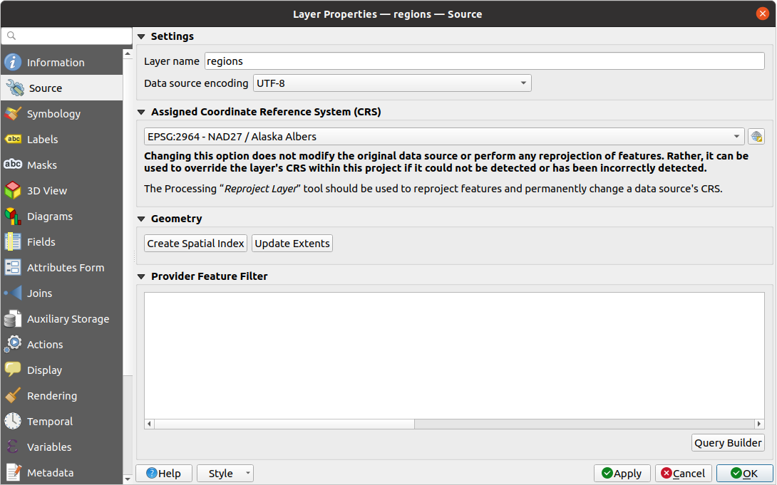
 Filter 아이콘이 나타납니다. 이 아이콘을 더블 클릭하면 Query Builder 대화창이 열려 쿼리를 편집할 수 있습니다. 쿼리 작성기 대화창은 메뉴를 통해서 열 수도 있습니다.
 Symbology 탭은 사용자 벡터 데이터를 렌더링하고 심볼 작업을 하기 위한 종합 도구를 제공합니다. 모든 벡터 데이터에 공통적으로 쓰이는 도구는 물론 서로 다른 벡터 데이터 유형에 맞춰 특화된 심볼 작업 도구도 이용할 수 있습니다. 하지만 모든 데이터 유형이 다음과 같은 대화창 구조를 공유합니다: 상단에는 범주화 및 피처에 적용할 심볼을 준비하는 데 쓰이는 위젯이, 하단에는 레이어 렌더링 위젯이 있습니다.
 Single Symbol 렌더링 작업자는 레이어의 모든 피처를 사용자가 정의한 단일 심볼을 이용해서 렌더링합니다. 심볼 표현에 대한 자세한 정보는 심볼 선택기 를 참조하세요.
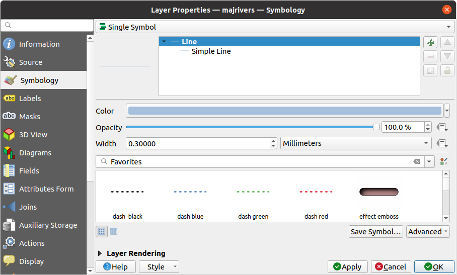
 No Symbols 렌더링 작업자는 모든 피처를 동일하게 렌더링하는 단일 심볼 렌더링 작업자의 특수한 용례입니다. 이 렌더링 작업자를 이용하면, 피처에 적용된 어떤 심볼도 렌더링하지 않지만 라벨, 도표 및 기타 심볼이 아닌 부분들은 렌더링될 것입니다.
 Categorized 렌더링 작업자는 필드 또는 표현식의 개별 값을 속성에 반영하는 사용자 지정 심볼을 이용해서 레이어의 피처를 렌더링합니다.
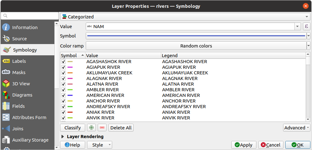
 버튼으로 작성할 수 있는 표현식 일 수도 있습니다. (예를 들어 사용자의 범주화 기준이 하나 이상의 속성으로부터 파생되는 경우) 범주화 작업에 표현식을 이용하면 심볼 범주화만을 위한 필드를 생성하지 않아도 됩니다.
 Random Color Ramp 임의의 색상표를 적용할 수 있습니다. 사용자가 만족하지 못 하는 경우 Shuffle Random Colors 를 클릭하면 새로운 임의의 색상 집합을 재생성할 수 있습니다.
 Add new categories,
  Remove
selected categories, Delete All of them or Delete Unused categories.
Remove
selected categories, Delete All of them or Delete Unused categories. Graduated 렌더링 작업자는 선택한 피처의 속성이 어떤 범주에 할당되는지를 반영하는 사용자 지정 심볼의 색상 또는 크기를 이용해서 레이어의 모든 피처를 렌더링합니다.
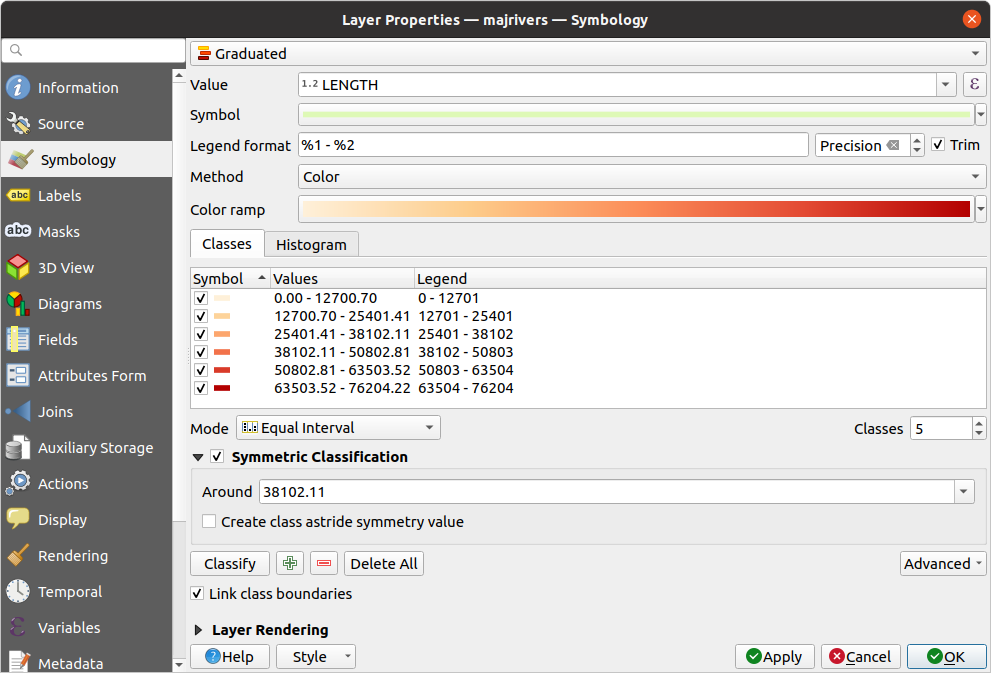
 Data-defined override 버튼 을 클릭하십시오.
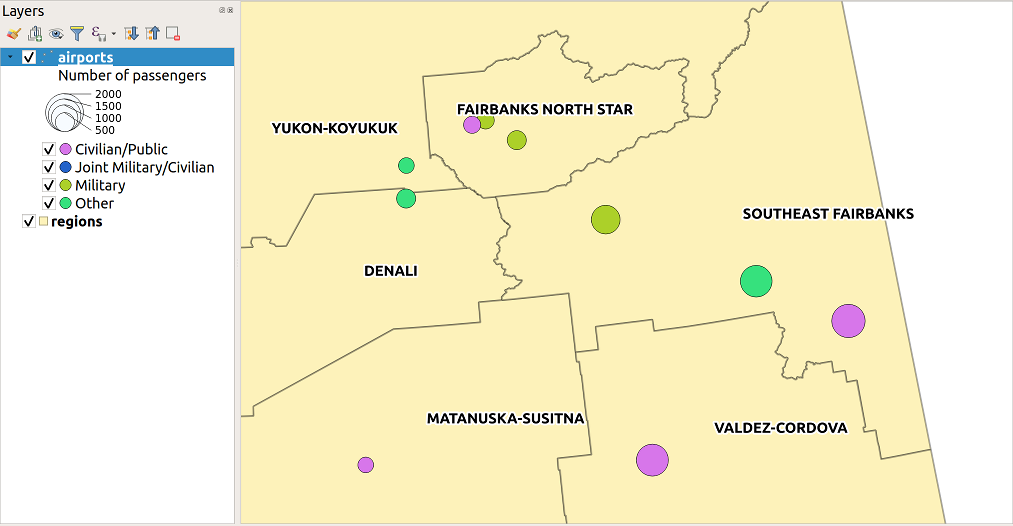
 Rule-based 렌더링 작업자는 선택한 피처를 세분화된 범주에 할당하는지를 반영하는 측면을 가진 심볼을 이용해서 레이어의 모든 피처를 렌더링하도록 설계되었습니다.
 Edit rule 또는
  Filter 옵션 옆에 있는 텍스트란에 표현식을 직접 입력하거나 그 옆에 있는
  Scale Range 옵션을 사용해서 규칙을 적용해야 할 축척을 설정할 수 있습니다.
 Else 옵션을 사용할 수 있습니다. 대화창의 규칙(Rule) 열에
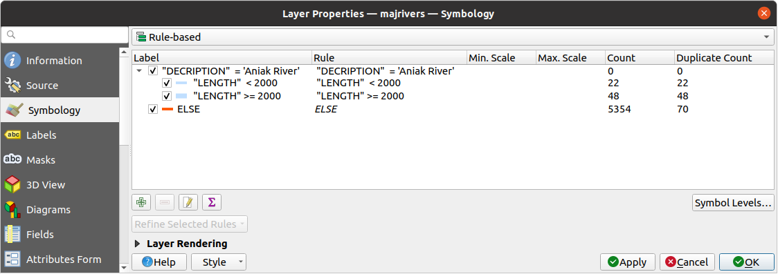
 Point Displacement 렌더링 작업자는 서로 지정한 허용 오차 거리에 들어오는 포인트 피처들을 받아서, 다양한 배치 방법에 따라 그 무게중심(barycenter) 주위에 심볼들을 배치합니다. 이 렌더링 작업자는 (예를 들어 같은 건물 안에 있는 오락시설들처럼) 포인트 레이어의 피처들이 동일한 위치에 존재하더라도 모두 가시화시킬 수 있는 편리한 방법이 될 수 있습니다.
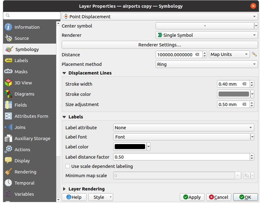
 Point Cluster 렌더링 작업자는 근접 포인트들을 단일하게 렌더링된 마커 심볼 하나로 그룹화합니다. 서로 특정 거리 안에 있는 포인트들을 단일 심볼로 병합하는 것이죠. 단순히 검색 거리 안에 있는 첫번째 그룹에 할당하기 보다는, 형성되는 그룹 가운데 가장 가까운 그룹을 기반으로 포인트 집합체를 생성합니다.
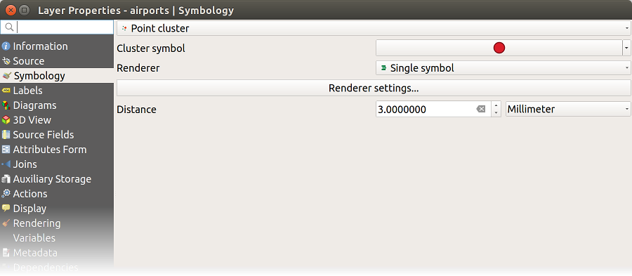
 Merged Features 렌더링 작업자는 복잡 심볼 또는 중첩하는 피처들을 균일하고 연속적인 지도 제작 심볼로 표현하기 위해 렌더링 전에 면(area)과 선(line) 피처들을 단일 객체로 “융합(dissolve)” 시킬 수 있습니다.
 Inverted Polygon 렌더링 작업자는 레이어에 있는 폴리곤의 바깥을 채울 심볼을 지정할 수 있습니다. 앞에서와 마찬가지로 단일 심볼, 등급, 범주, 규칙 기반 또는 2.5D 같은 하위 렌더링 작업자를 선택할 수 있습니다.
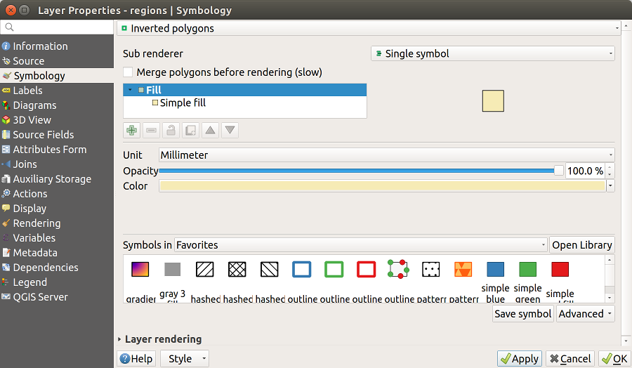
 Heatmap renderer you can create live
dynamic heatmaps for (multi)point layers.
You can specify the heatmap Radius in millimeters, points, pixels, map units or
inches, choose and edit a Color ramp for the heatmap style and use a slider for
selecting a trade-off between render speed and quality. You can also define a
Maximum value limit and Weight points by using a field or an expression.
Heatmap renderer you can create live
dynamic heatmaps for (multi)point layers.
You can specify the heatmap Radius in millimeters, points, pixels, map units or
inches, choose and edit a Color ramp for the heatmap style and use a slider for
selecting a trade-off between render speed and quality. You can also define a
Maximum value limit and Weight points by using a field or an expression.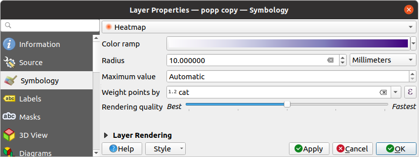
 2.5D 렌더링 작업자를 이용해서 사용자 레이어의 피처에 2.5D 효과를 줄 수 있습니다. 먼저 Height 값(맵 단위)을 설정하십시오. 고정값, 사용자 레이어의 필드 가운데 하나, 또는 표현식으로 설정할 수 있습니다. 또 시각의 방향을 (0° 는 서쪽으로, 값이 올라갈수록 반시계 방향으로 돕니다) 재현하려면 Angle (도 단위)을 설정해야 합니다. Roof Color 및 Wall Color 을 설정하려면 고급 환경 설정 옵션을 사용하십시오. 만약 피처의 벽에 태양광 효과를 주고 싶다면,
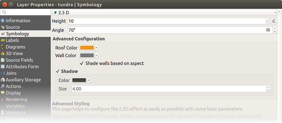
 : 이 도구를 통해 맵 캔버스에서 아래에 있는 레이어를 가시화할 수 있습니다. 슬라이드 바를 통해 사용자 벡터 레이어의 가시성을 필요에 따라 조정하십시오. 슬라이드 바 옆에 있는 메뉴에서 가시성을 정확한 백분율로 설정할 수도 있습니다.
 버튼을 클릭하십시오. Define Order 대화창이 열리는데, 다음 작업들을 할 수 있습니다:
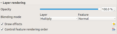

 Draw Effects 옵션은 사용자가 벡터 레이어의 가시화를 직접 조정할 수 있도록 그리기 효과를 추가합니다.
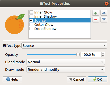
 Grayscale 을 통해 회색조 심볼을 어떻게 생성할지 (‘By lightness’, ‘By luminosity’, ‘By average’ 그리고 ‘Off’ 옵션 가운데 하나를) 선택할 수 있습니다.
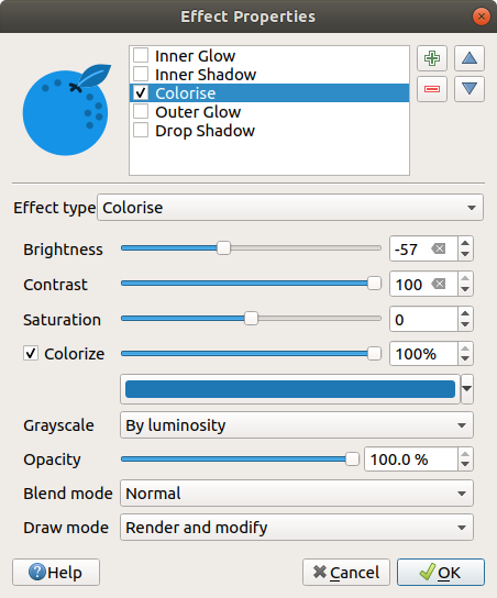
 Move up 및
  Move down 버튼으로 효과의 순서를 바꿀 수 있고,
  Labels 속성 대화창은 벡터 레이어에 대해 스마트 라벨 작업 환경을 설정하기 위해 필요한 그리고 적절한 모든 기능을 제공합니다. Layer Styling 패널에서 또는 라벨 툴바 의
  Configure project labeling rules button:
helps you control interactions between labels and features across the layers in the project.
More details at Configuring project labeling rules.
Configure project labeling rules button:
helps you control interactions between labels and features across the layers in the project.
More details at Configuring project labeling rules. Automated placement settings (applies to all layers) button:
configure general properties on label placement and conflicts resolution.
More details at 자동화된 배치 엔진 설정하기.
Automated placement settings (applies to all layers) button:
configure general properties on label placement and conflicts resolution.
More details at 자동화된 배치 엔진 설정하기. No labels: 기본값입니다. 레이어에 어떤 라벨도 표시하지 않습니다.
 Blocking: 어떤 레이어의 라벨을 렌더링하지 않고 해당 레이어가 다른 레이어를 가리도록만 설정할 수 있습니다.
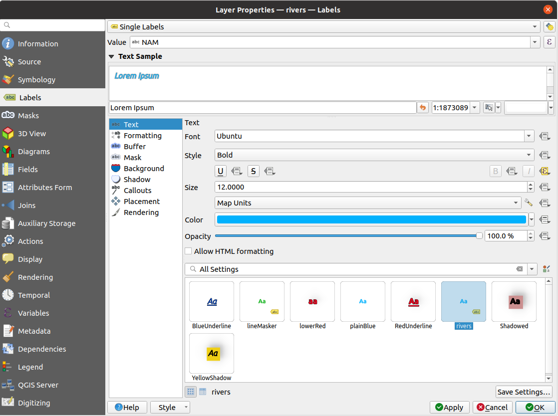


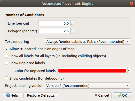
 규칙 기반 라벨 작업 을 선택하십시오.
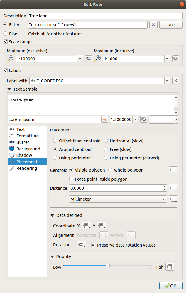
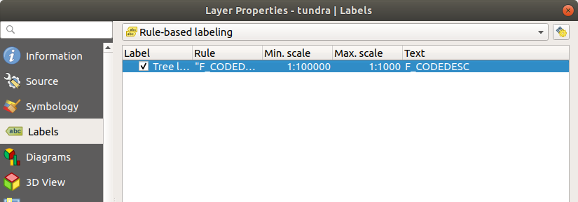
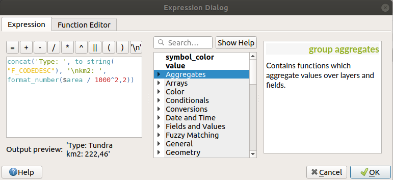
 으로 바뀝니다.
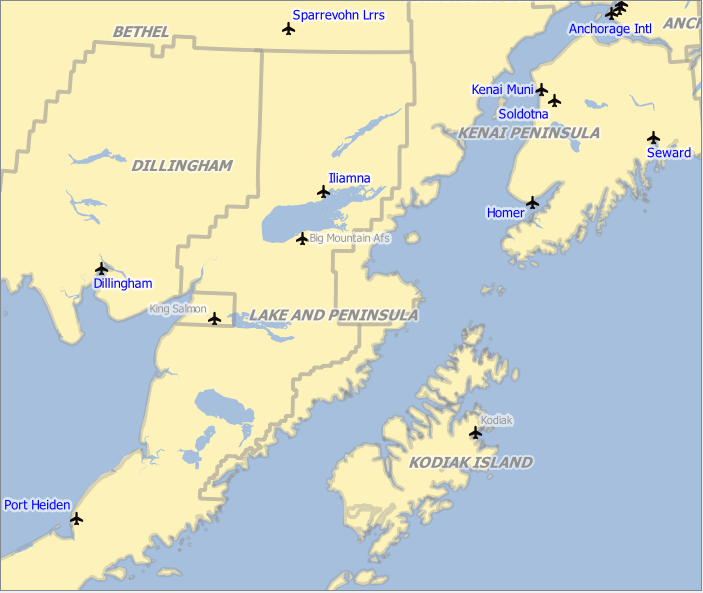
 렌더링,
렌더링,  도표 속성을 조작할 수 있는 몇몇 도구를 제공합니다:
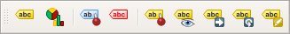
 Highlight Pinned Labels, Diagrams and Callouts: 라벨 항목이 속한 벡터 레이어가 편집 가능 상태인 경우 녹색으로 강조되고, 편집 가능 상태가 아니라면 파란색을 유지합니다.
 Toggle Display of Unplaced Labels: 어떤 중요한 라벨이 (예를 들면 중첩 또는 다른 제약조건 때문에) 맵에서 누락되었는지 여부를 확인할 수 있습니다. 이런 라벨은 사용자 지정이 가능한 색상으로 표시됩니다. (자동화된 배치 엔진 설정하기 를 참조하세요.)
 Pin/Unpin Labels and Diagrams. By clicking or dragging an
area, you pin overlaid items. If you click or drag an area holding Shift,
the items are unpinned. Finally, you can also click or drag an area holding
Ctrl to toggle their pin status.
Pin/Unpin Labels and Diagrams. By clicking or dragging an
area, you pin overlaid items. If you click or drag an area holding Shift,
the items are unpinned. Finally, you can also click or drag an area holding
Ctrl to toggle their pin status. Show/Hide Labels and Diagrams: 항목을 클릭하거나 kbd:Shift 키를 누른 채 어떤 영역을 클릭&드래그하면 해당 항목을 숨깁니다. 항목이 숨겨져 있는 경우, 그냥 해당 피처를 한번 클릭하면 가시성을 복원합니다. 영역을 드래그하면 해당 영역에 있는 모든 항목의 가시성을 복원할 것입니다.
 Move a Label, Diagram or Callout: 항목을 클릭해서 선택한 다음 원하는 위치를 클릭해서 해당 위치로 옮깁니다. 새로운 좌표는 보조 필드 에 저장됩니다. 이 도구로 항목을 선택한 다음 Delete 키를 누르면 저장된 위치값을 삭제할 것입니다.
 Rotate a Label: 라벨을 클릭해서 선택한 다음 원하는 기울기가 적용되도록 다시 클릭하십시오. 마찬가지로, 새 각도는 보조 필드에 저장됩니다. 이 도구로 라벨을 선택한 다음 Delete 키를 누르면 해당 라벨의 기울기값을 삭제할 것입니다.
 Change Label Properties: 이 아이콘을 누른 다음 라벨을 클릭하면, 해당 라벨의 속성을 변경할 수 있는 대화창이 열립니다. 라벨 그 자체, 라벨의 좌표, 각도, 글꼴, 크기, 멀티라인 정렬 등등 그 속성이 필드에 매핑돼 있는 한 해당 속성을 변경할 수 있습니다. 여기에서 피처의 모든 부분에 라벨을 붙이는
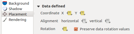
 Toggle Editing 버튼으로 레이어를 편집 가능한 상태로 설정합니다.
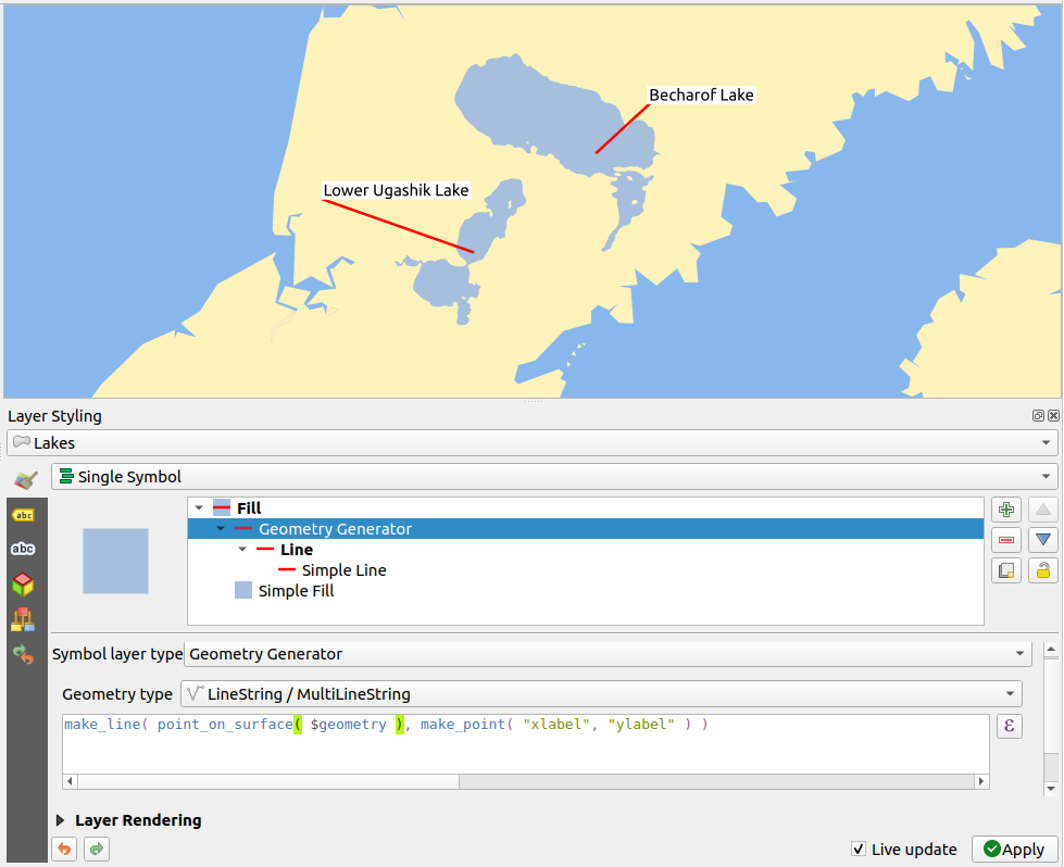
 No diagrams: 기본값입니다. 피처 위로 어떤 도표도 표시하지 않습니다.
 Pie chart: 원형 통계 그래픽인 원형 차트로, 숫자로 나타낸 비율을 보여주는 조각들로 나누어집니다. 각 조각의 원호 길이는 각 조각이 나타내는 양과 비례합니다.
 Text diagram, a horizontally divided circle showing statistic
values inside;
Text diagram, a horizontally divided circle showing statistic
values inside; Histogram, bars of varying colors for each attribute
aligned next to each other;
Histogram, bars of varying colors for each attribute
aligned next to each other; Stacked bars, stacks bars of varying colors for each
attribute on top of each other vertically or horizontally;
Stacked bars, stacks bars of varying colors for each
attribute on top of each other vertically or horizontally; Stacked diagram, stacks diagrams of equal or varying
types, next to each other, vertically or horizontally. More details at
Stacked Diagrams.
Stacked diagram, stacks diagrams of equal or varying
types, next to each other, vertically or horizontally. More details at
Stacked Diagrams.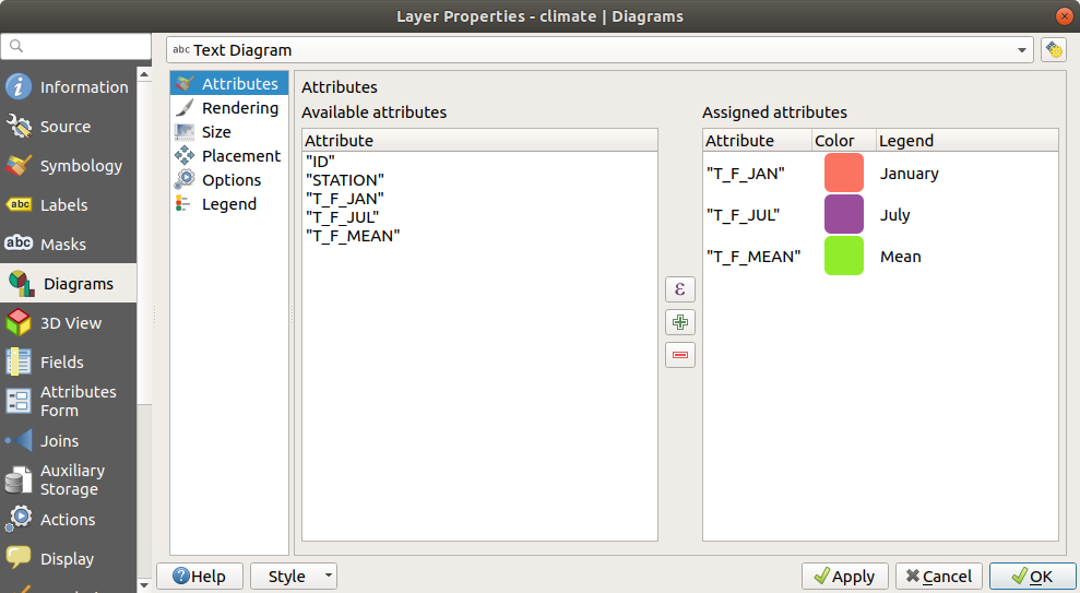
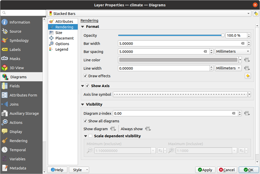
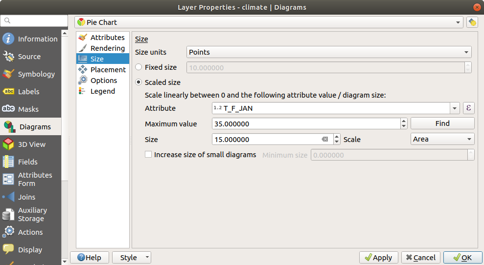
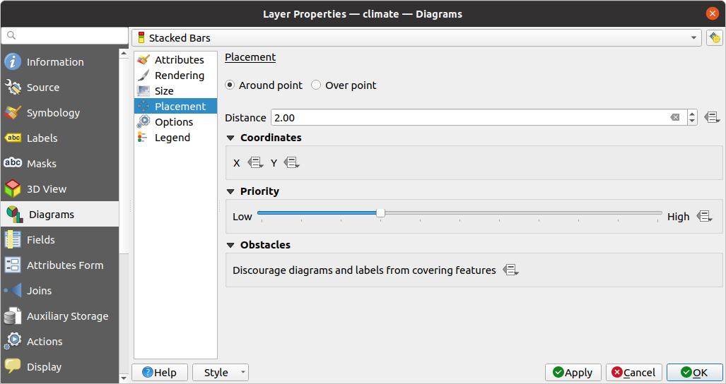

 Masks 탭에서 다른 모든 레이어의 심볼 레이어 또는 라벨과 중첩하는 현재 레이어 심볼을 환경 설정할 수 있습니다. 즉 중첩하는 경우 색상이 비슷해 구분하기 힘든 심볼 및 라벨의 가독성을 향상시킬 수 있다는 뜻입니다. 항목 주변에 사용자 지정한 투명 마스크를 추가해서 현재 레이어의 심볼 레이어의 일부분을 “숨깁니다”.
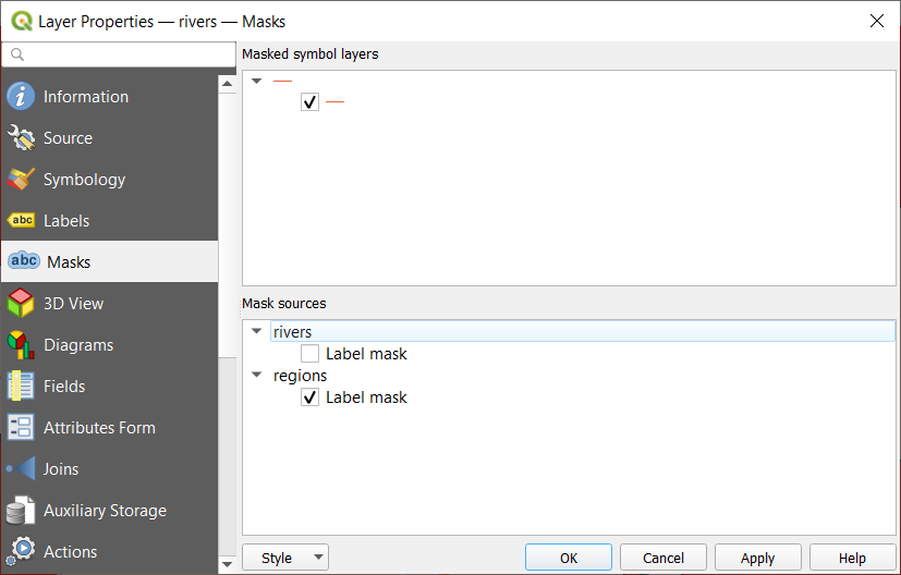
 3D View 탭은 3D 맵 뷰 도구에서 묘사되어야 할 벡터 레이어를 위한 설정을 제공합니다.
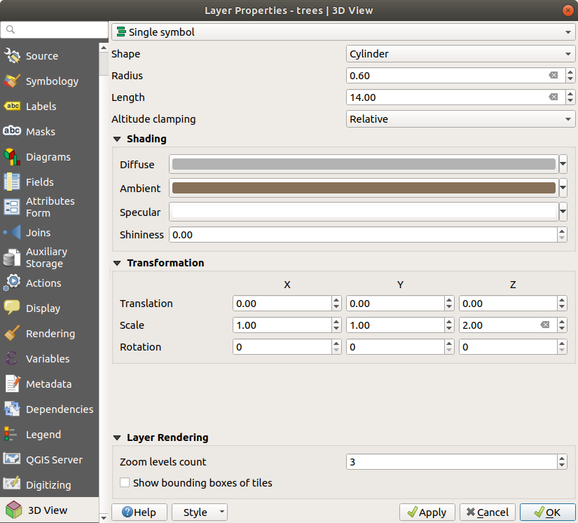
 Fields 탭은 레이어 관련 필드에 대한 정보를 제공하며, 레이어 필드를 정리할 수 있습니다.
 New field 및
  Delete field 버튼을 사용해서 레이어 구조를 수정할 수 있습니다.
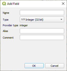
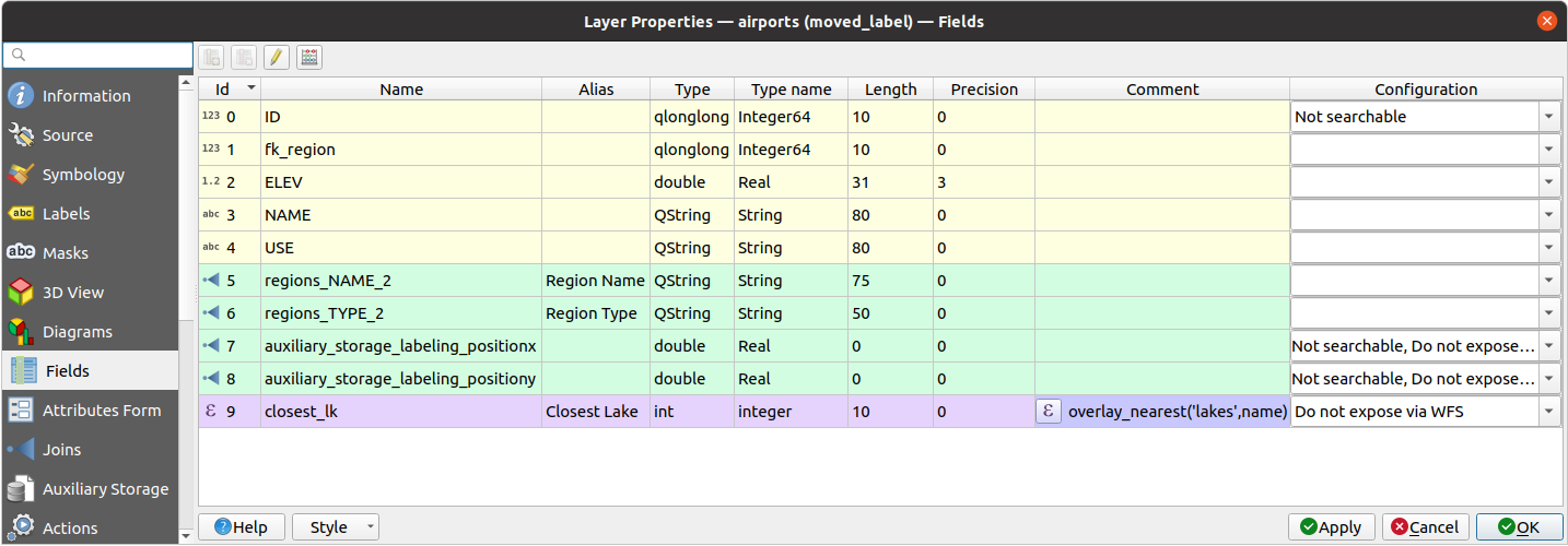
 Attributes Form tab helps you set up the form to
display when creating new features, editing or querying existing one.
This affects them in both table and form views.
You can define:
Attributes Form tab helps you set up the form to
display when creating new features, editing or querying existing one.
This affects them in both table and form views.
You can define: Identify Features 도구로 피처를 클릭하거나 또는 속성 테이블을 양식 뷰(form view) 모드로 바꾸는 경우, 기본적으로 QGIS는 기본 양식을 미리 정의된 위젯과 함께 표시합니다. (일반적으로 스핀박스(spinbox)와 텍스트 상자로 이루어집니다. 지정된 행에 각 필드를 위젯 옆에 있는 필드 라벨로 표현합니다.) 만약 레이어에 관계 가 설정돼 있다면, 양식의 하단에 내장된 프레임에 참조 레이어의 필드를 동일한 기본 구조대로 표시합니다.
 Show field aliases instead of names button allows
you to toggle field aliases and field names.
Show field aliases instead of names button allows
you to toggle field aliases and field names.
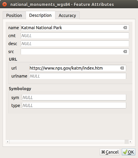
 Invert selection 버튼으로 선택한 필드를 반전시킬 수 있습니다.
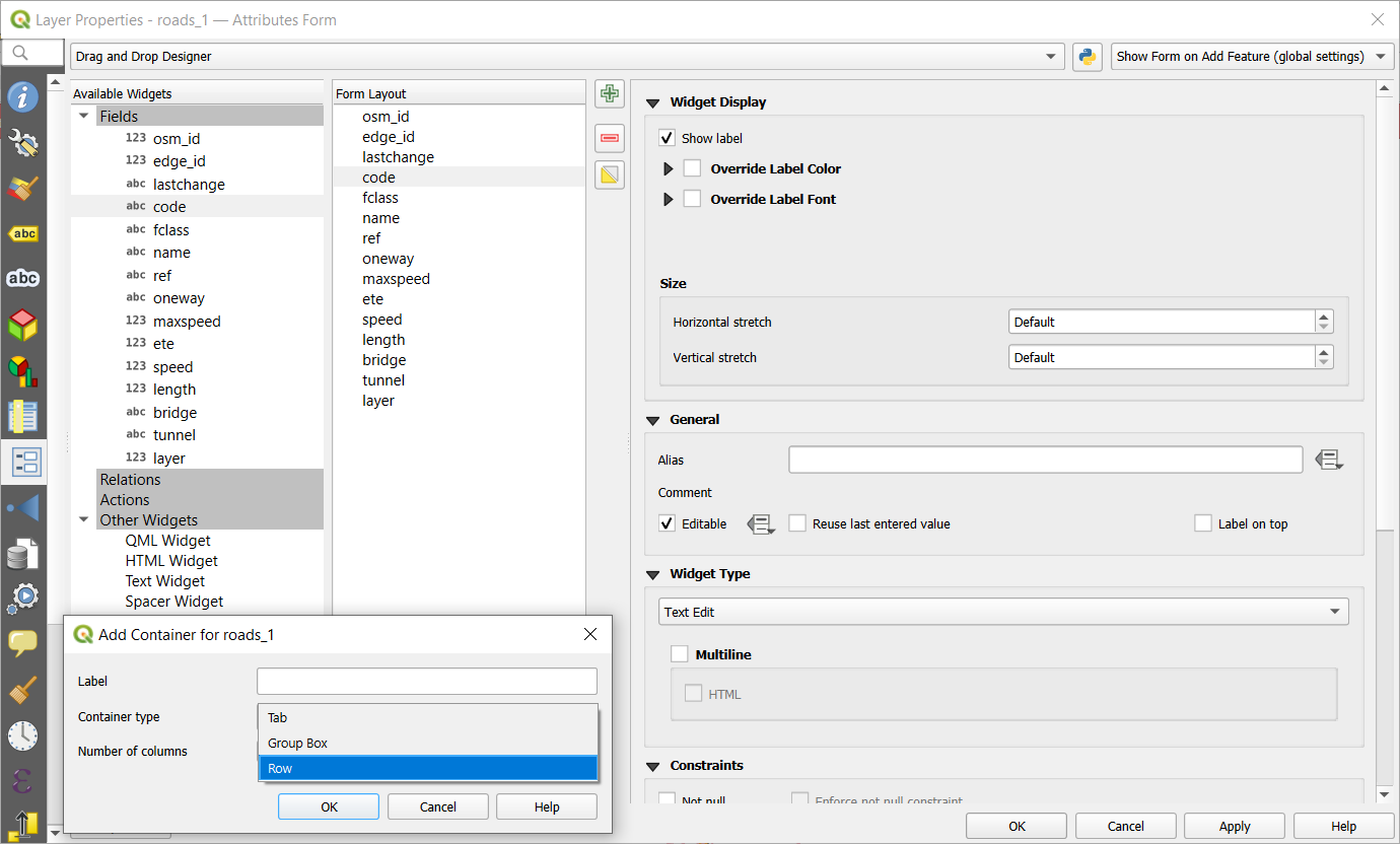

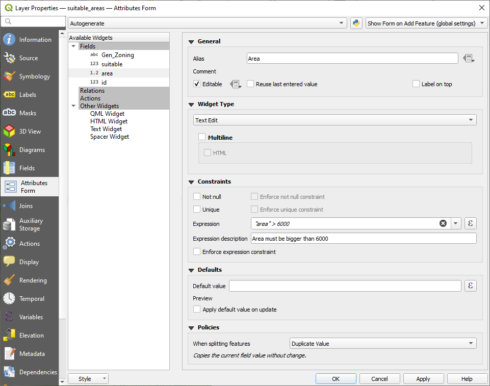
 Joins 탭에서, 현재 레이어의 피처와 또다른 불러온 벡터 레이어의 (또는 테이블의) 피처를 결합시킬 수 있습니다. 결합은 레이어들이 1대1 관계로 공유하는 속성을 기반으로 합니다. 결합에 대해 더 자세히 알고 싶다면 두 레이어 간 피처 결합하기 를 읽어보세요.
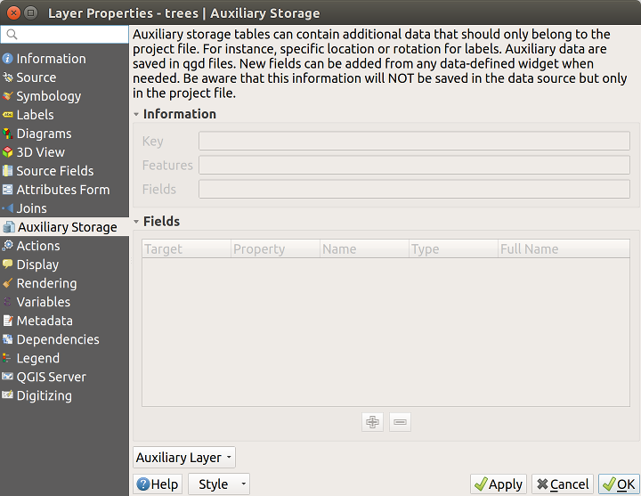
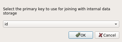
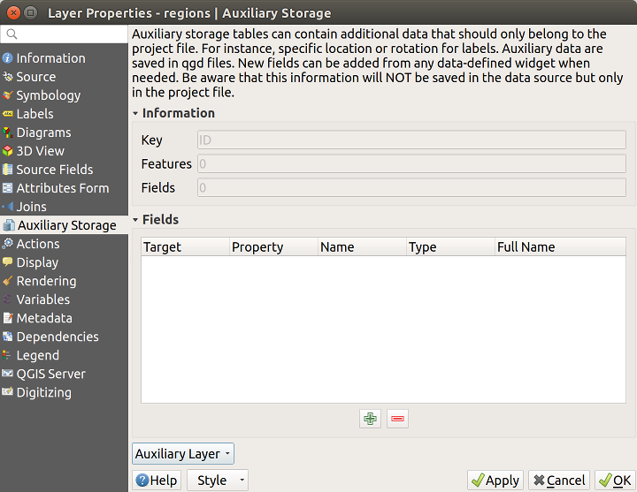
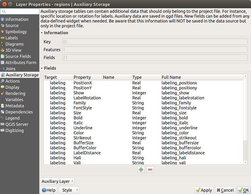
 아이콘이 표시된 것을 눈치채셨나요? 데이터 정의 무시 옵션이 정확하게 설정되었다는 의미입니다:
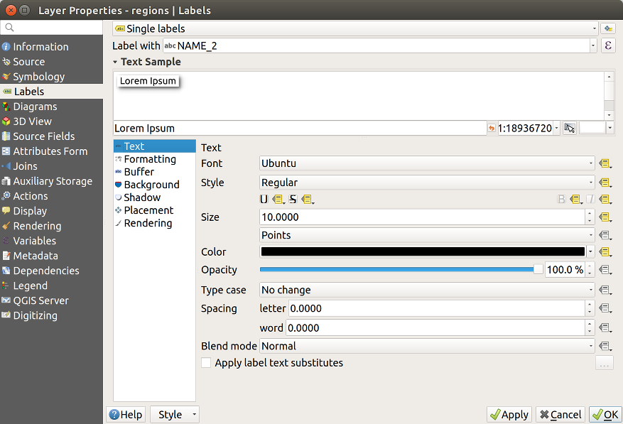
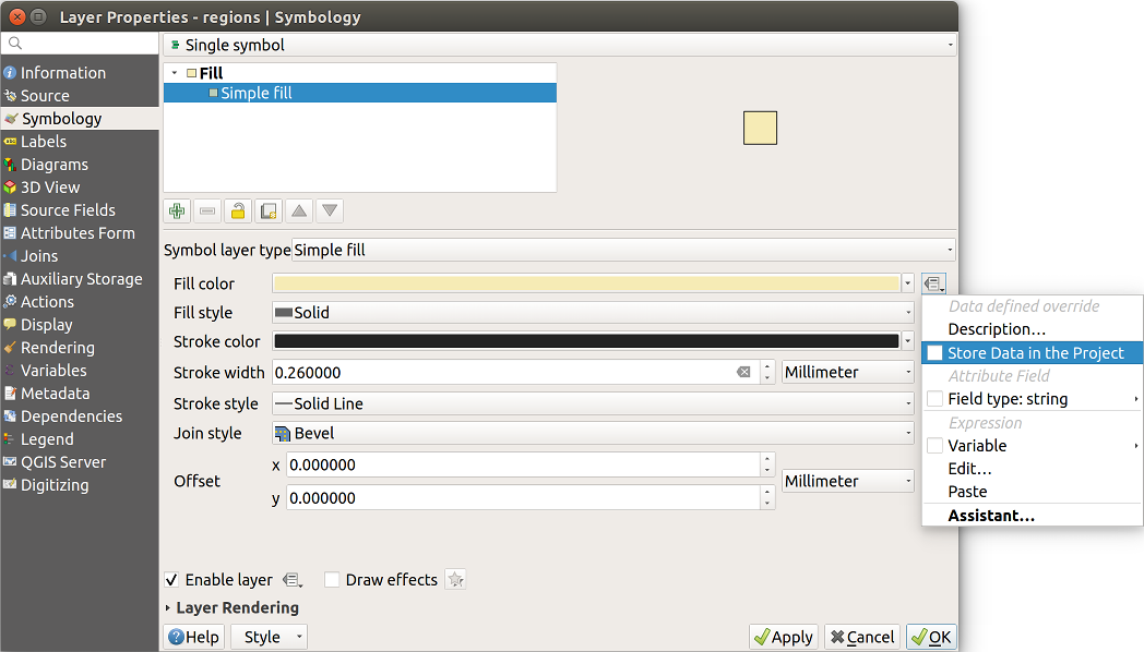
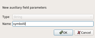
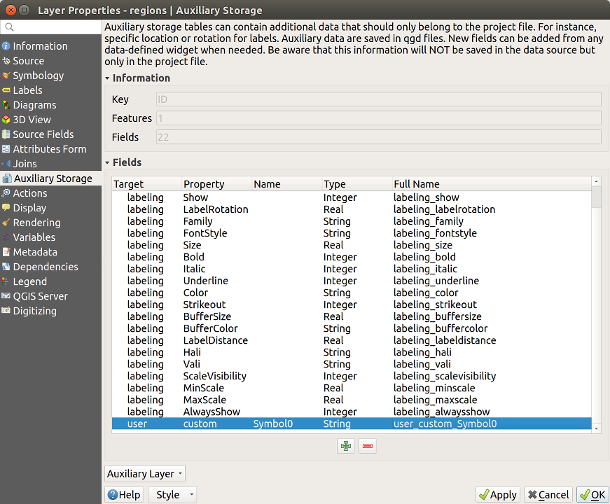
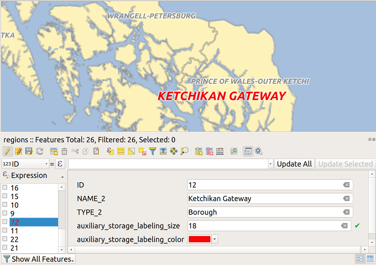
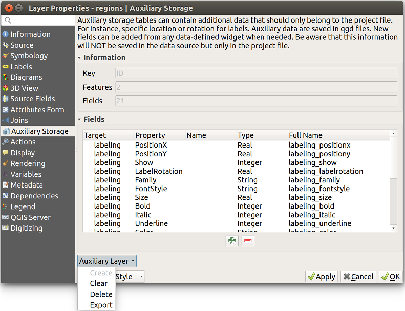
 Actions 탭은 객체의 속성을 기반으로 하는 액션을 수행할 수 있는 기능을 제공하고 있습니다. 예를 들면 객체의 속성에서 생성한 인자(argument)와 함께 프로그램을 실행하거나 또는 웹 보고 도구에 파라미터를 전달하는 등의 수많은 액션을 수행할 수 있습니다.
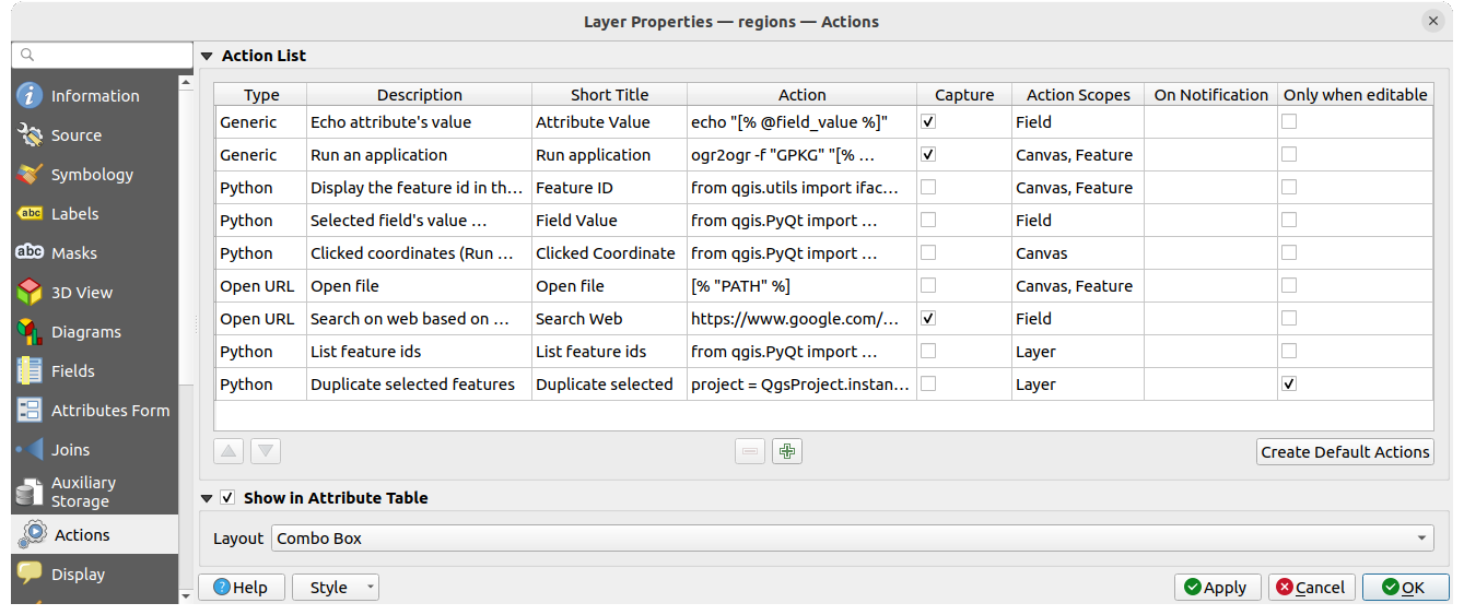
 Duplicate an action
to open the Duplicate Action dialog. You must have selected at least one existing action
in order to create a duplicate.
Duplicate an action
to open the Duplicate Action dialog. You must have selected at least one existing action
in order to create a duplicate. Run Feature Action 버튼의 드롭다운 메뉴를 통해
 또는 아마도
  에서만 동작할 겁니다) 벡터 레이어에서 데이터를 추출해서 파일로 삽입하는 또다른 예시가 있습니다. 이 레이어는 수종명
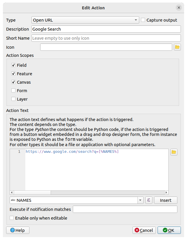
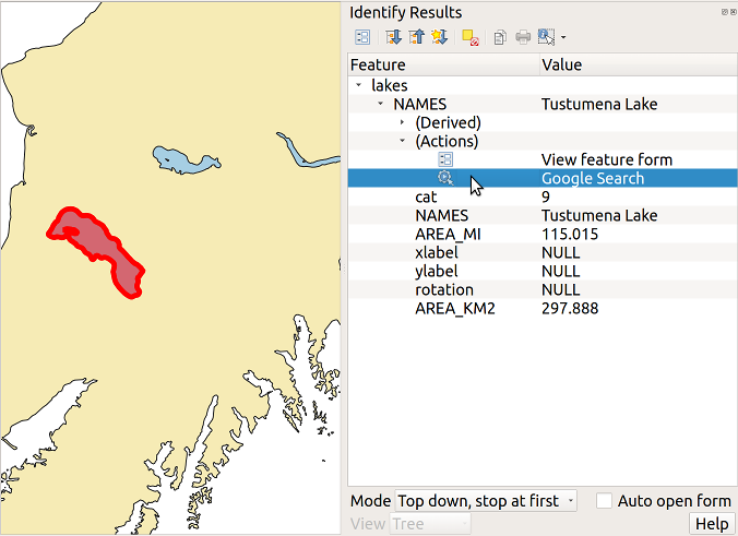
 Display 탭에서 피처 식별에 사용되는 필드의 환경을 설정할 수 있습니다:
 Show Map Tips 아이콘을 누른 상태에서 활성화된 레이어의 피처 위에 마우스를 가져갔을 때 맵 캔버스에 표시되는 메시지.
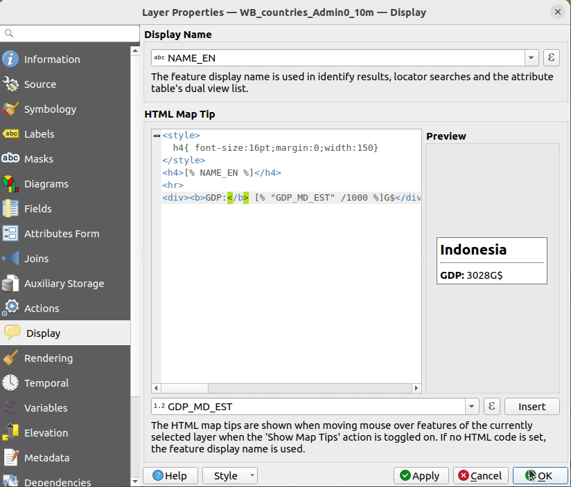
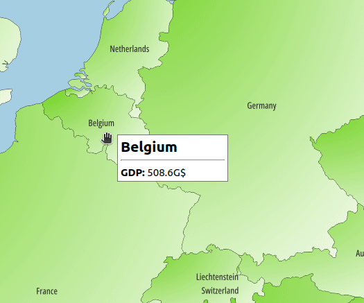
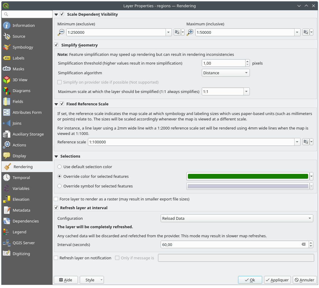
 Rendering 탭에서 다음 설정을 할 수 있습니다:
 Set to current canvas scale 버튼을 클릭하면 현재 맵 캔버스의 축척을 가시성 범위의 한계값으로 설정할 수 있습니다. 자세한 내용은 가시성 축척 선택기 을 참조하세요.
 Temporal 탭은 레이어의 렌더링을 시간에 따라 제어할 수 있는 옵션들을 제공합니다. 이런 동적 렌더링에는 맵 캔버스 전체에 적용되는 시계열 탐색 을 활성화해야 할 필요가 있습니다.
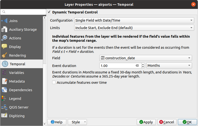
 Elevation 탭은 3차원 맵 뷰 안에서의 레이어 표고 속성 및 단면 도구 도표(profile tool charts) 에서의 3차원 맵 뷰의 모양을 제어할 수 있는 옵션들을 제공합니다. 그 중에서도 다음을 설정할 수 있습니다:
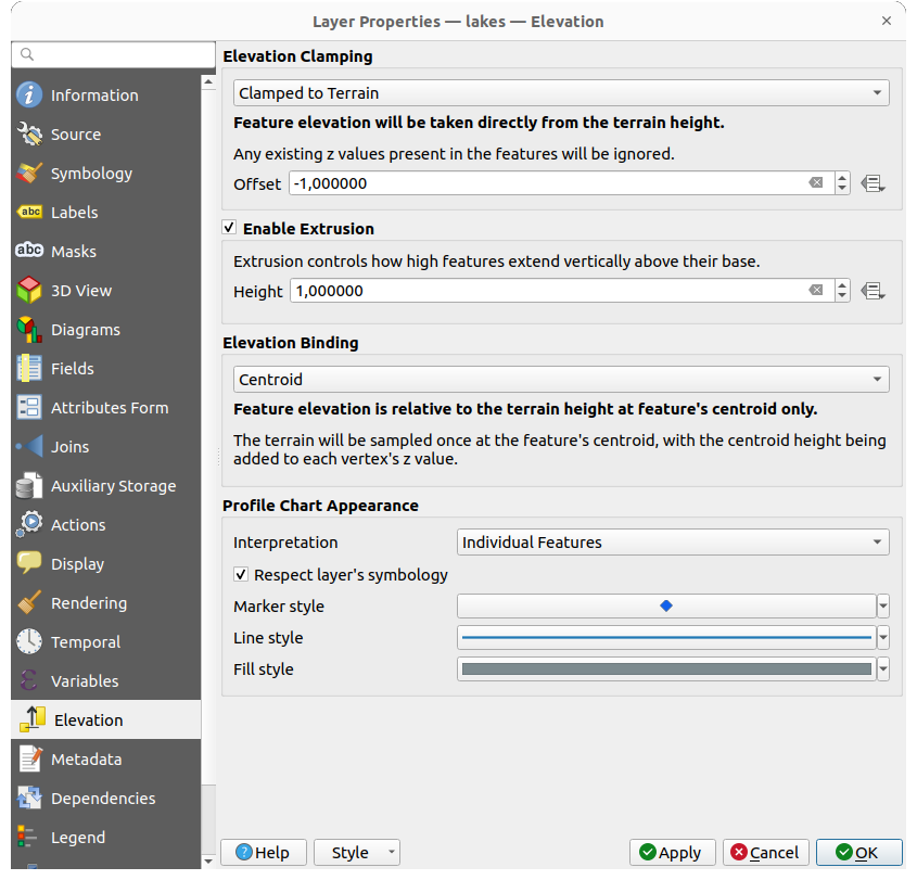
 Select CRS.
Vertical reference systems are supported for vector layers by:
Select CRS.
Vertical reference systems are supported for vector layers by: Metadata 탭에 사용자 레이어에 대한 메타데이터 리포트를 생성하고 편집할 수 있는 옵션이 있습니다. 더 자세한 정보는 메타데이터 를 참조하세요.
 Dependencies 탭에서 레이어 사이의 데이터 의존성을 선언할 수 있습니다. 레이어에서 ─ 사용자가 직접 수정하지 않고 ─ 데이터가 수정되면 다른 레이어의 데이터가 수정될 수도 있는 경우 데이터 의존성이 발생합니다. 예를 들면 레이어의 도형을 수정한 후 데이터베이스 트리거 또는 사용자 지정 PyQGIS 스크립트 작업이 또다른 레이어의 도형을 업데이트하는 경우를 말합니다.
 Legend 속성 탭은 레이어 패널 그리고/또는 인쇄 조판기 범례 를 위한, 다음과 같은 옵션을 포함하는 고급 설정을 제공합니다:
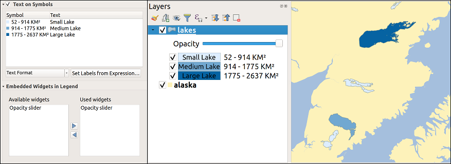
 QGIS Server 탭은 Description, Attribution, Metadata URL, 그리고 Legend URL 부분들로 이루어져 있습니다.
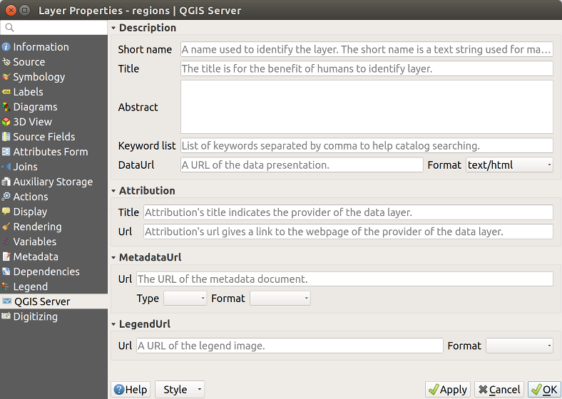
 Digitizing 탭은 디지타이즈한 도형의 질을 보장하도록 하는 옵션들을 제공합니다.
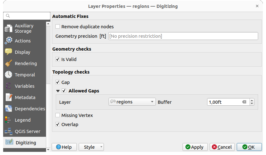
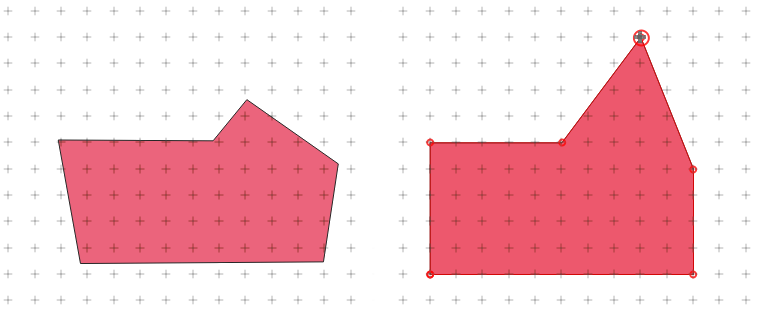
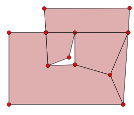
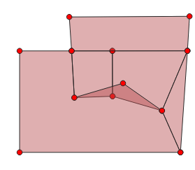
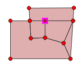
 Zoom to Feature(s): 피처(들)로 확대/축소
 Zoom to problem: 오류 위치로 확대/축소