중요

번역은 여러분이 참여할 수 있는 커뮤니티 활동입니다. 이 페이지는 현재 66.67% 번역되었습니다.

17.15. 래스터 레이어 잘라내기 및 병합하기

참고

이 수업에서는 계속 실제 세상의 시나리오 안에서 공간 알고리즘을 사용해서 공간 데이터를 준비하는 또다른 예제를 풀어볼 것입니다.

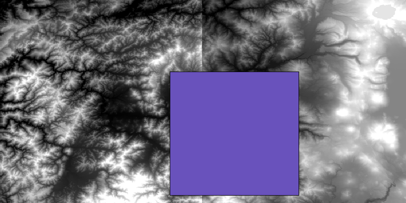
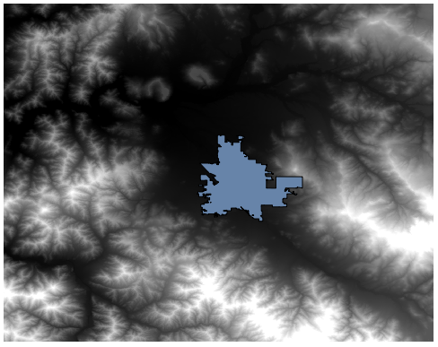
이 수업에서는, 단일 폴리곤으로 이루어진 벡터 레이어로부터 도시 지역을 둘러싼 영역의 경사도 레이어를 계산해보겠습니다. 기본 DEM은 래스터 레이어 두 개로 나뉘어져 있습니다. 이 두 레이어를 함께 사용해야만 우리가 작업하고자 하는 도시 주변 영역보다 더 넓은 영역을 커버하게 됩니다. 이 수업에 해당하는 프로젝트를 열어보면, 다음과 같은 화면을 보게 될 것입니다.

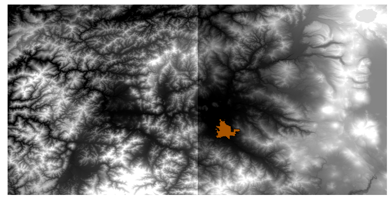
이 레이어들은 두 가지 문제점을 가지고 있습니다:

• 우리가 원하는 것보다 (우리의 관심 지역은 도심을 둘러싼 좁은 영역입니다) 너무 넓은 지역을 커버하고 있습니다.

• 서로 다른 파일 두 개로 되어 있습니다. (도시의 범위는 래스터 레이어 가운데 하나에 들어가지만, 앞에서 언급했듯이 주변에 더 넓은 범위를 원합니다.)

적합한 공간 알고리즘을 사용한다면 두 문제점 모두 쉽게 해결할 수 있습니다.

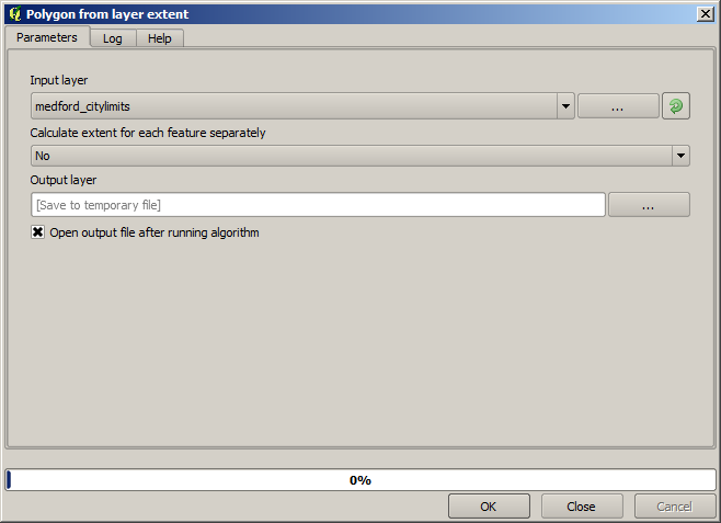
먼저, 우리가 원하는 영역을 정의하는 사각형을 생성하십시오. 이를 위해 도시 지역의 경계를 나타내는 경계 상자(bounding box)를 담고 있는 레이어를 생성하고, 꼭 필요한 것보다 조금 더 넓은 영역을 커버하는 래스터 레이어를 얻기 위한 버퍼를 지정하십시오.

To calculate the bounding box , we can use the Extract layer extent algorithm

To buffer it, we use the Buffer algorithm, with the following parameter values.

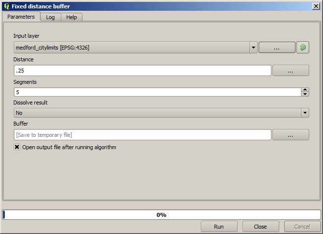
경고

최신 버전에서는 문법이 바뀌었습니다. 거리와 원호 꼭짓점 모두 0.25로 설정하세요.

이 파라미터 값을 통해 다음과 같은 경계 상자 결과물을 얻을 수 있습니다.

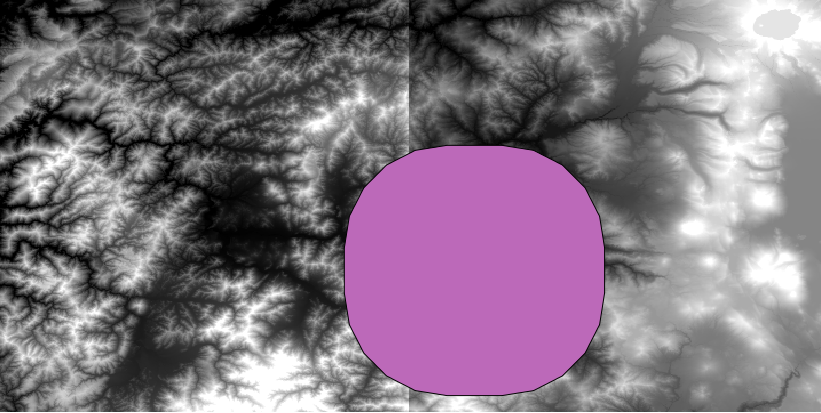
It is a rounded box, but we can easily get the equivalent box with square angles, by running the Extract layer extent algorithm on it. We could have buffered the city limits first, and then calculate the extent rectangle, saving one step.

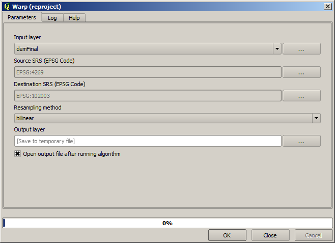
You will notice that the rasters has a different projection from the vector. We should therefore reproject them before proceeding further, using the Warp (reproject) tool.

참고

최신 버전의 인터페이스는 좀 더 복잡합니다. 적어도 하나 이상의 압축 방법을 선택했는지 확인하세요.

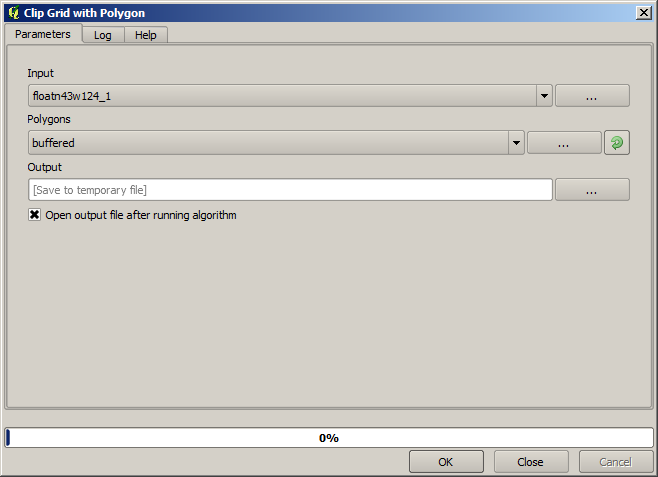
With this layer that contains the bounding box of the raster layer that we want to obtain, we can crop both of the raster layers, using the Clip raster by mask layer algorithm.

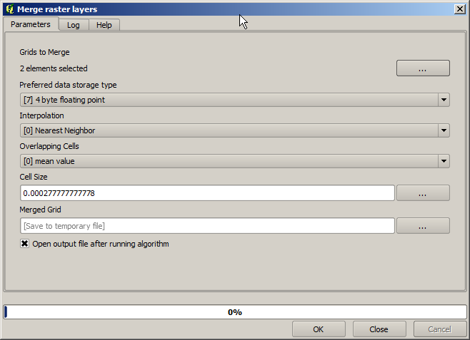
Once the layers have been cropped, they can be merged using the SAGA Mosaic raster layers algorithm.

참고

병합을 먼저 하고 잘라내면 잘라내기 알고리즘을 두 번 호출할 필요가 없어 시간을 절약할 수 있습니다. 하지만 병합해야 할 레이어가 두 개 이상인데 용량이 큰 편일 경우, 병합을 먼저 하면 나중에 처리하기 어려워질 수가 있습니다. 이런 경우 잘라내기 알고리즘을 몇 번 호출해야만 해서 시간이 걸릴 수도 있지만, 곧 이런 작업을 자동화할 수 있는 추가 도구들을 소개할 것이므로 걱정하지 마십시오. 이 예제에서는 레이어 두 개뿐이므로 이런 상황에 대해 걱정할 필요는 없습니다.

병합 작업으로 결국 원하는 DEM을 얻게 되었습니다.

이제 경사도 레이어를 계산할 시간입니다.

A slope layer can be computed with the Slope algorithm, but the DEM obtained in the last step is not suitable as input, since elevation values are in meters but cellsize is not expressed in meters (the layer uses a CRS with geographic coordinates). A reprojection is needed. To reproject a raster layer, the Warp (reproject) algorithm can be used again. We reproject into a CRS with meters as units (e.g. 3857), so we can then correctly calculate the slope, with either SAGA or GDAL.

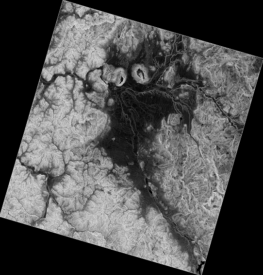
이 새 DEM을 써서 경사를 계산할 수 있습니다.

다음이 결과물인 경사도 레이어입니다.

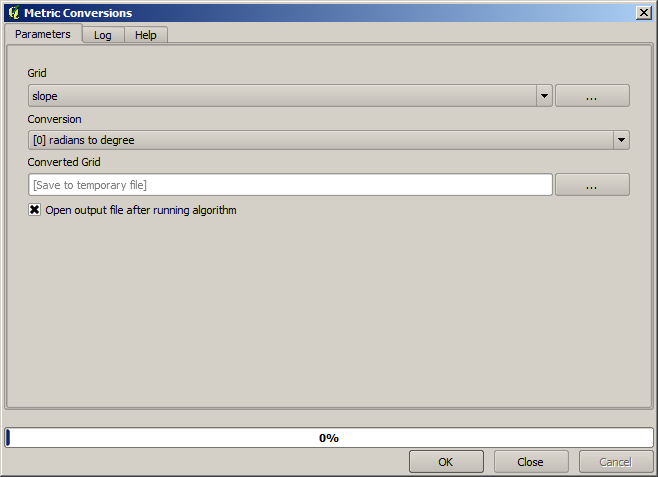
The slope produced by the Slope algorithm can be expressed in degrees or radians; degrees are a more practical and common unit. In case you calculated it in radians, the Metric conversions algorithm will help us to do the conversion (but in case you didn’t know that algorithm existed, you could use the raster calculator that we have already used).

Reprojecting the converted slope layer back with the Reproject raster layer, we get the final layer we wanted.

재투영 과정에서 최종 레이어가 초기 단계에서 계산했던 경계 상자 바깥에 값을 가지게 될 수도 있습니다. 기본 DEM을 얻기 위해 했던 것과 동일한 방법으로 다시 잘라내면 이 문제를 해결할 수 있습니다.