Coordinate Reference Systems
|
Objectives: |
Understanding of Coordinate Reference Systems. |
Keywords: |
Coordinate Reference System (CRS), Map Projection, On the Fly Projection, Latitude, Longitude, Northing, Easting |
Overview
Map projections try to portray the surface of the earth or a portion of the earth on a flat piece of paper or computer screen. In a lay man’s term, map projections tries to transform the earth from its spherical shape (3D) to a planar shape (2D) so that maps can be made on flat layers e.g maps.
A coordinate reference system (CRS) then defines, with the help of coordinates, how the two-dimensional, projected map in your GIS is related to real places on the earth. The decision as to which map projection and coordinate reference system to use, depends on the regional extent of the area you want to work in, on the analysis you want to do and often on the availability of data.
Map Projection in detail
A traditional method of representing the earth’s shape is the use of globes. There is, however, a problem with this approach. Although globes preserve the majority of the earth’s shape and illustrate the spatial configuration of continent-sized features, they are very difficult to carry in one’s pocket. They are also only convenient to use at extremely small scales (e.g. 1:100 million).
Most of the thematic map data commonly used in GIS applications are of considerably larger scale. Typical GIS datasets have scales of 1:250 000 or greater, depending on the level of detail. A globe of this size would be difficult and expensive to produce and even more difficult to carry around. As a result, cartographers have developed a set of techniques called map projections designed to show, with reasonable accuracy, the spherical earth in two-dimensions.
When viewed at close range the earth appears to be relatively flat. However when viewed from space, we can see that the earth is relatively spherical. Maps, as we will see in the upcoming map production topic, are representations of reality. They are designed to not only represent features, but also their shape and spatial arrangement. Each map projection has advantages and disadvantages. The best projection for a map depends on the scale of the map, and on the purposes for which it will be used. For example, a projection may have unacceptable distortions if used to map the entire African continent, but may be an excellent choice for a large-scale (detailed) map of your country. The properties of a map projection may also influence some of the design features of the map. Some projections are good for small areas, some are good for mapping areas with a large East-West extent, and some are better for mapping areas with a large North-South extent.
The three families of map projections
The process of creating map projections is best illustrated by positioning a light source inside a transparent globe on which opaque earth features are placed. Then project the feature outlines onto a two-dimensional flat piece of paper. Different ways of projecting can be produced by surrounding the globe in a cylindrical fashion, as a cone, or even as a flat surface. Each of these methods produces what is called a map projection family. Therefore, there is a family of planar projections, a family of cylindrical projections, and another called conical projections (see figure_projection_families)
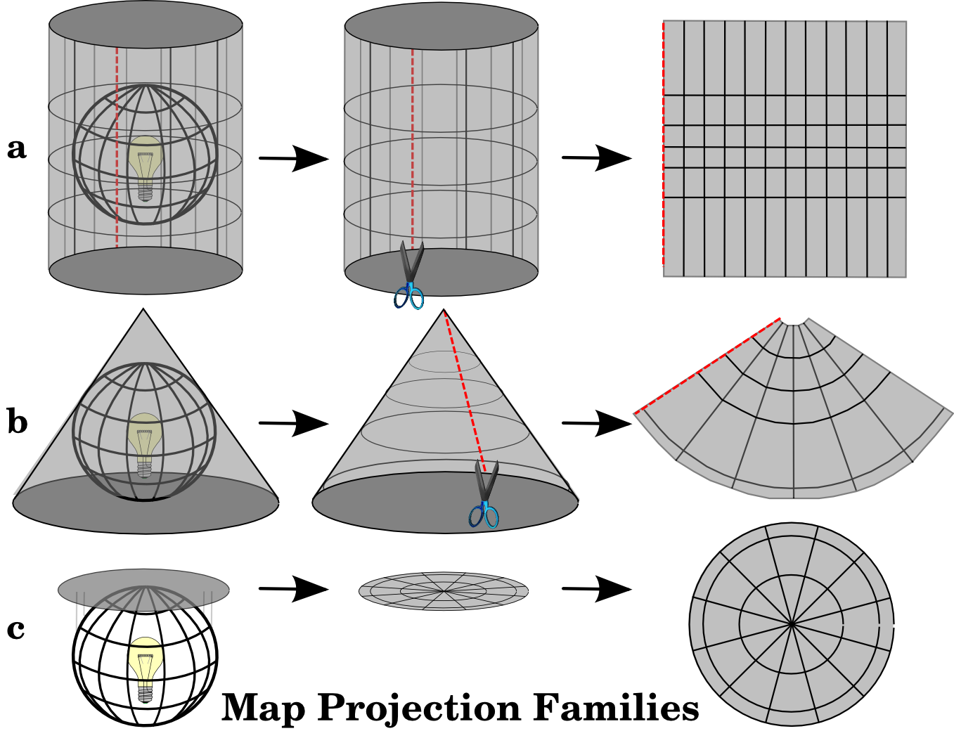
The three families of map projections. They can be represented by a) cylindrical projections, b) conical projections or c) planar projections.
Today, of course, the process of projecting the spherical earth onto a flat piece of paper is done using the mathematical principles of geometry and trigonometry. This recreates the physical projection of light through the globe.
Accuracy of map projections
Map projections are never absolutely accurate representations of the spherical earth. As a result of the map projection process, every map shows distortions of angular conformity, distance and area. A map projection may combine several of these characteristics, or may be a compromise that distorts all the properties of area, distance and angular conformity, within some acceptable limit. Examples of compromise projections are the Winkel Tripel projection and the Robinson projection (see figure_robinson_projection), which are often used for producing and visualizing world maps.
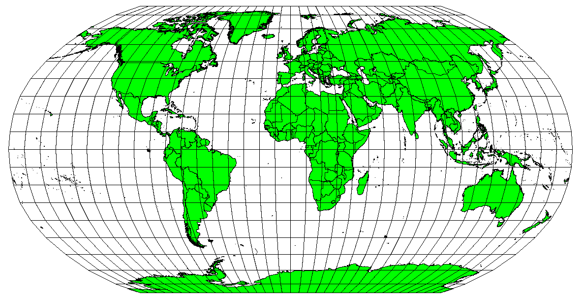
The Robinson projection is a compromise where distortions of area, angular conformity and distance are acceptable.
It is usually impossible to preserve all characteristics at the same time in a map projection. This means that when you want to carry out accurate analytical operations, you need to use a map projection that provides the best characteristics for your analyses. For example, if you need to measure distances on your map, you should try to use a map projection for your data that provides high accuracy for distances.
Map projections with angular conformity
When working with a globe, the main directions of the compass rose (North, East, South and West) will always occur at 90 degrees to one another. In other words, East will always occur at a 90 degree angle to North. Maintaining correct angular properties can be preserved on a map projection as well. A map projection that retains this property of angular conformity is called a conformal or orthomorphic projection.
These projections are used when the preservation of angular relationships is important. They are commonly used for navigational or meteorological tasks. It is important to remember that maintaining true angles on a map is difficult for large areas and should be attempted only for small portions of the earth. The conformal type of projection results in distortions of areas, meaning that if area measurements are made on the map, they will be incorrect. The larger the area the less accurate the area measurements will be. Examples are the Mercator projection (as shown in figure_mercator_projection) and the Lambert Conformal Conic projection. The U.S. Geological Survey uses a conformal projection for many of its topographic maps.
The Mercator projection, for example, is used where angular relationships are important, but the relationship of areas are distorted.
Map projections with equal distance
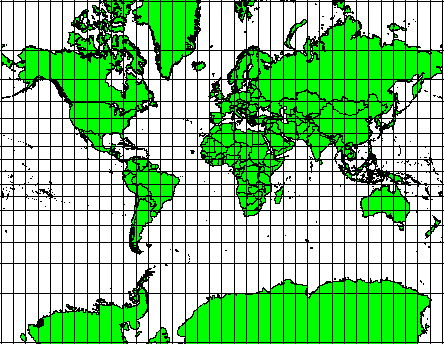
If your goal in projecting a map is to accurately measure distances, you should select a projection that is designed to preserve distances well. Such projections, called equidistant projections, require that the scale of the map is kept constant. A map is equidistant when it correctly represents distances from the centre of the projection to any other place on the map. Equidistant projections maintain accurate distances from the centre of the projection or along given lines. These projections are used for radio and seismic mapping, and for navigation. The Plate Carree Equidistant Cylindrical (see figure_plate_caree_projection) and the Equirectangular projection are two good examples of equidistant projections. The Azimuthal Equidistant projection is the projection used for the emblem of the United Nations (see figure_azimuthal_equidistant_projection).
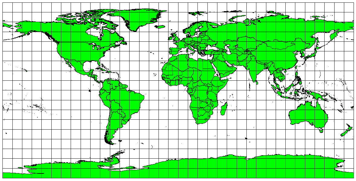
The Plate Carree Equidistant Cylindrical projection, for example, is used when accurate distance measurement is important.

The United Nations Logo uses the Azimuthal Equidistant projection.
Projections with equal areas
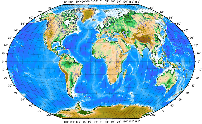
When a map portrays areas over the entire map, so that all mapped areas have the same proportional relationship to the areas on the Earth that they represent, the map is an equal area map. In practice, general reference and educational maps most often require the use of equal area projections. As the name implies, these maps are best used when calculations of area are the dominant calculations you will perform. If, for example, you are trying to analyse a particular area in your town to find out whether it is large enough for a new shopping mall, equal area projections are the best choice. On the one hand, the larger the area you are analysing, the more precise your area measures will be, if you use an equal area projection rather than another type. On the other hand, an equal area projection results in distortions of angular conformity when dealing with large areas. Small areas will be far less prone to having their angles distorted when you use an equal area projection. Alber’s equal area, Lambert’s equal area and Mollweide Equal Area Cylindrical projections (shown in figure_mollweide_equal_area_projection) are types of equal area projections that are often encountered in GIS work.

The Mollweide Equal Area Cylindrical projection, for example, ensures that all mapped areas have the same proportional relationship to the areas on the Earth.
Keep in mind that map projection is a very complex topic. There are hundreds of different projections available world wide each trying to portray a certain portion of the earth’s surface as faithfully as possible on a flat piece of paper. In reality, the choice of which projection to use, will often be made for you. Most countries have commonly used projections and when data is exchanged people will follow the national trend.
Coordinate Reference System (CRS) in detail
With the help of coordinate reference systems (CRS) every place on the earth can be specified by a set of three numbers, called coordinates. In general CRS can be divided into projected coordinate reference systems (also called Cartesian or rectangular coordinate reference systems) and geographic coordinate reference systems.
Geographic Coordinate Systems
The use of Geographic Coordinate Reference Systems is very common. They use degrees of latitude and longitude and sometimes also a height value to describe a location on the earth’s surface. The most popular is called WGS 84.
Lines of latitude run parallel to the equator and divide the earth into 180 equally spaced sections from North to South (or South to North). The reference line for latitude is the equator and each hemisphere is divided into ninety sections, each representing one degree of latitude. In the northern hemisphere, degrees of latitude are measured from zero at the equator to ninety at the north pole. In the southern hemisphere, degrees of latitude are measured from zero at the equator to ninety degrees at the south pole. To simplify the digitisation of maps, degrees of latitude in the southern hemisphere are often assigned negative values (0 to -90°). Wherever you are on the earth’s surface, the distance between the lines of latitude is the same (60 nautical miles). See figure_geographic_crs for a pictorial view.
Geographic coordinate system with lines of latitude parallel to the equator and lines of longitude with the prime meridian through Greenwich.
Lines of longitude, on the other hand, do not stand up so well to the standard of uniformity. Lines of longitude run perpendicular to the equator and converge at the poles. The reference line for longitude (the prime meridian) runs from the North pole to the South pole through Greenwich, England. Subsequent lines of longitude are measured from zero to 180 degrees East or West of the prime meridian. Note that values West of the prime meridian are assigned negative values for use in digital mapping applications. See figure_geographic_crs for a pictorial view.
At the equator, and only at the equator, the distance represented by one line of longitude is equal to the distance represented by one degree of latitude. As you move towards the poles, the distance between lines of longitude becomes progressively less, until, at the exact location of the pole, all 360° of longitude are represented by a single point that you could put your finger on (you probably would want to wear gloves though). Using the geographic coordinate system, we have a grid of lines dividing the earth into squares that cover approximately 12363.365 square kilometres at the equator — a good start, but not very useful for determining the location of anything within that square.
To be truly useful, a map grid must be divided into small enough sections so that
they can be used to describe (with an acceptable level of accuracy) the location
of a point on the map. To accomplish this, degrees are divided into minutes
(') and seconds ("). There are sixty minutes in a degree, and sixty
seconds in a minute (3600 seconds in a degree). So, at the equator, one second
of latitude or longitude = 30.87624 meters.
Projected coordinate reference systems
A two-dimensional coordinate reference system is commonly defined by two axes. At right angles to each other, they form a so called XY-plane (see figure_projected_crs on the left side). The horizontal axis is normally labelled X, and the vertical axis is normally labelled Y. In a three-dimensional coordinate reference system, another axis, normally labelled Z, is added. It is also at right angles to the X and Y axes. The Z axis provides the third dimension of space (see figure_projected_crs on the right side). Every point that is expressed in spherical coordinates can be expressed as an X Y Z coordinate.
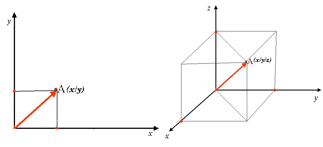
Two and three dimensional coordinate reference systems.
A projected coordinate reference system in the southern hemisphere (south of the equator) normally has its origin on the equator at a specific Longitude. This means that the Y-values increase southwards and the X-values increase to the West. In the northern hemisphere (north of the equator) the origin is also the equator at a specific Longitude. However, now the Y-values increase northwards and the X-values increase to the East. In the following section, we describe a projected coordinate reference system, called Universal Transverse Mercator (UTM) often used for South Africa.
Universal Transverse Mercator (UTM) CRS in detail
The Universal Transverse Mercator (UTM) coordinate reference system has its origin on the equator at a specific Longitude. Now the Y-values increase southwards and the X-values increase to the West. The UTM CRS is a global map projection. This means, it is generally used all over the world. But as already described in the section ‘accuracy of map projections’ above, the larger the area (for example South Africa) the more distortion of angular conformity, distance and area occur. To avoid too much distortion, the world is divided into 60 equal zones that are all 6 degrees wide in longitude from East to West. The UTM zones are numbered 1 to 60, starting at the international date line (zone 1 at 180 degrees West longitude) and progressing East back to the international date line (zone 60 at 180 degrees East longitude) as shown in figure_utm_zones.
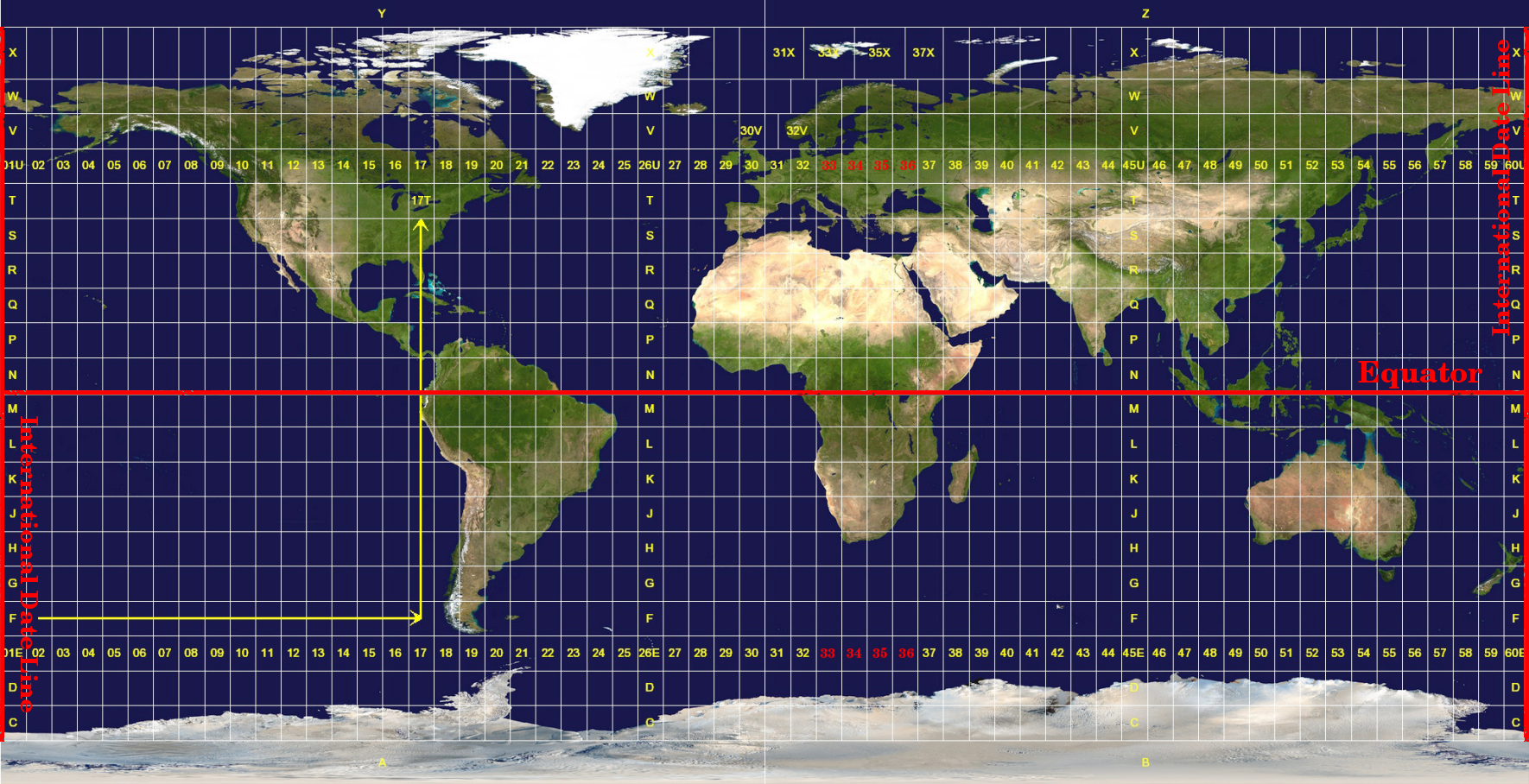
The Universal Transverse Mercator zones. For South Africa UTM zones 33S, 34S, 35S, and 36S are used.
As you can see in figure_utm_zones and figure_utm_for_sa, South Africa is covered by four UTM zones to minimize distortion. The zones are called UTM 33S, UTM 34S, UTM 35S and UTM 36S. The S after the zone means that the UTM zones are located south of the equator.
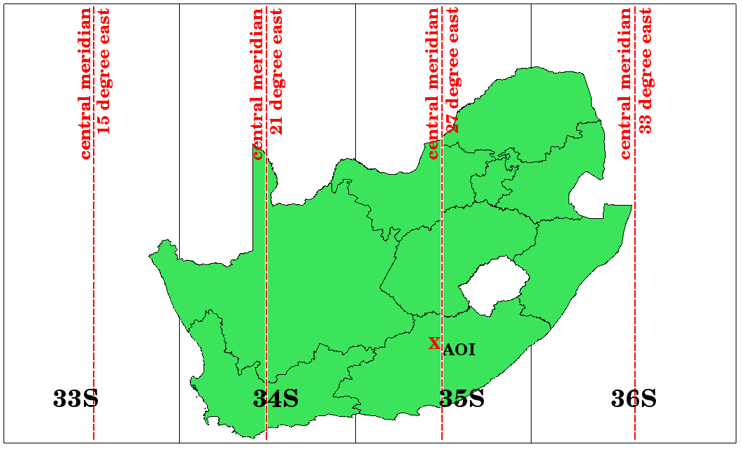
UTM zones 33S, 34S, 35S, and 36S with their central longitudes (meridians) used to project South Africa with high accuracy. The red cross shows an Area of Interest (AOI).
Say, for example, that we want to define a two-dimensional coordinate within the Area of Interest (AOI) marked with a red cross in figure_utm_for_sa. You can see, that the area is located within the UTM zone 35S. This means, to minimize distortion and to get accurate analysis results, we should use UTM zone 35S as the coordinate reference system.
The position of a coordinate in UTM south of the equator must be indicated with the zone number (35) and with its northing (Y) value and easting (X) value in meters. The northing value is the distance of the position from the equator in meters. The easting value is the distance from the central meridian (longitude) of the used UTM zone. For UTM zone 35S it is 27 degrees East as shown in figure_utm_for_sa. Furthermore, because we are south of the equator and negative values are not allowed in the UTM coordinate reference system, we have to add a so called false northing value of 10,000,000 m to the northing (Y) value and a false easting value of 500,000 m to the easting (X) value. This sounds difficult, so, we will do an example that shows you how to find the correct UTM 35S coordinate for the Area of Interest.
The northing (Y) value
The place we are looking for is 3,550,000 meters south of the equator, so the northing (Y) value gets a negative sign and is -3,550,000 m. According to the UTM definitions we have to add a false northing value of 10,000,000 m. This means the northing (Y) value of our coordinate is 6,450,000 m (-3,550,000 m + 10,000,000 m).
The easting (X) value
First we have to find the central meridian (longitude) for the UTM zone 35S. As we can see in figure_utm_for_sa it is 27 degrees East. The place we are looking for is 85,000 meters West from the central meridian. Just like the northing value, the easting (X) value gets a negative sign, giving a result of -85,000 m. According to the UTM definitions we have to add a false easting value of 500,000 m. This means the easting (X) value of our coordinate is 415,000 m (-85,000 m + 500,000 m). Finally, we have to add the zone number to the easting value to get the correct value.
As a result, the coordinate for our Point of Interest, projected in UTM zone 35S would be written as: 35 415,000 m E / 6,450,000 m N. In some GIS, when the correct UTM zone 35S is defined and the units are set to meters within the system, the coordinate could also simply appear as 415,000 6,450,000.
On-The-Fly Projection
As you can probably imagine, there might be a situation where the data you want to use in a GIS are projected in different coordinate reference systems. For example, you might get a vector layer showing the boundaries of South Africa projected in UTM 35S and another vector layer with point information about rainfall provided in the geographic coordinate system WGS 84. In GIS these two vector layers are placed in totally different areas of the map window, because they have different projections.
To solve this problem, many GIS include a functionality called on-the-fly projection. It means, that you can define a certain projection when you start the GIS and all layers that you then load, no matter what coordinate reference system they have, will be automatically displayed in the projection you defined. This functionality allows you to overlay layers within the map window of your GIS, even though they may be in different reference systems.
Common problems / things to be aware of
The topic map projection is very complex and even professionals who have studied geography, geodetics or any other GIS related science, often have problems with the correct definition of map projections and coordinate reference systems. Usually when you work with GIS, you already have projected data to start with. In most cases these data will be projected in a certain CRS, so you don’t have to create a new CRS or even re project the data from one CRS to another. That said, it is always useful to have an idea about what map projection and CRS means.
What have we learned?
Let’s wrap up what we covered in this worksheet:
Map projections portray the surface of the earth on a two-dimensional, flat piece of paper or computer screen.
There are global map projections, but most map projections are created and optimized to project smaller areas of the earth’s surface.
Map projections are never absolutely accurate representations of the spherical earth. They show distortions of angular conformity, distance and area. It is impossible to preserve all these characteristics at the same time in a map projection.
A Coordinate reference system (CRS) defines, with the help of coordinates, how the two-dimensional, projected map is related to real locations on the earth.
There are two different types of coordinate reference systems: Geographic Coordinate Systems and Projected Coordinate Systems.
On the Fly projection is a functionality in GIS that allows us to overlay layers, even if they are projected in different coordinate reference systems.
Now you try!
Here are some ideas for you to try with your learners:
Start QGIS and load two layers of the same area but with different projections and let your pupils find the coordinates of several places on the two layers. You can show them that it is not possible to overlay the two layers. Then define the coordinate reference system as Geographic/WGS 84 inside the Project Properties dialog and activate the checkbox
 Enable on-the-fly CRS transformation. Load the two layers of the
same area again and let your pupils see how on-the-fly projection works.
Enable on-the-fly CRS transformation. Load the two layers of the
same area again and let your pupils see how on-the-fly projection works.You can open the Project Properties dialog in QGIS and show your pupils the many different Coordinate Reference Systems so they get an idea of the complexity of this topic. With ‘on-the-fly’ CRS transformation enabled you can select different CRS to display the same layer in different projections.
Something to think about
If you don’t have a computer available, you can show your pupils the principles of the three map projection families. Get a globe and paper and demonstrate how cylindrical, conical and planar projections work in general. With the help of a transparency sheet you can draw a two-dimensional coordinate reference system showing X axes and Y axes. Then, let your pupils define coordinates (X and Y values) for different places.
Further reading
Books:
Chang, Kang-Tsung (2006). Introduction to Geographic Information Systems. 3rd Edition. McGraw Hill. ISBN: 0070658986
DeMers, Michael N. (2005). Fundamentals of Geographic Information Systems. 3rd Edition. Wiley. ISBN: 9814126195
Galati, Stephen R. (2006): Geographic Information Systems Demystified. Artech House Inc. ISBN: 158053533X
Websites:
https://www.colorado.edu/geography/gcraft/notes/mapproj/mapproj_f.html
https://geology.isu.edu/wapi/geostac/Field_Exercise/topomaps/index.htm
The QGIS User Guide also has more detailed information on working with map projections in QGIS.
What’s next?
In the section that follows we will take a closer look at Map Production.