16.2. Working with the Attribute Table
The attribute table displays information on features of a selected layer. Each row in the table represents a feature (with or without geometry), and each column contains a particular piece of information about the feature. Features in the table can be searched, selected, moved or even edited.
16.2.1. Foreword: Spatial and non-spatial tables
QGIS allows you to load spatial and non-spatial layers. This currently includes tables supported by GDAL and delimited text, as well as the PostgreSQL, MS SQL Server, SpatiaLite and Oracle providers. All loaded layers are listed in the Layers panel. Whether a layer is spatially enabled or not determines whether you can interact with it on the map.
Non-spatial tables can be browsed and edited using the attribute table view. Furthermore, they can be used for field lookups. For example, you can use columns of a non-spatial table to define attribute values, or a range of values that are allowed, to be added to a specific vector layer during digitizing. Have a closer look at the edit widget in section Attributes Form Properties to find out more.
16.2.2. Introducing the attribute table interface
To open the attribute table for a vector layer, activate the layer by
clicking on it in the Layers Panel. Then, from the main
menu, choose  . It is also possible to right-click on the layer and choose
from the drop-down menu,
or to click on the Open Attribute Table button
in the Attributes toolbar.
If you prefer shortcuts, F6 will open the attribute table.
Shift+F6 will open the attribute table filtered to selected features and
Ctrl+F6 will open the attribute table filtered to visible features.
. It is also possible to right-click on the layer and choose
from the drop-down menu,
or to click on the Open Attribute Table button
in the Attributes toolbar.
If you prefer shortcuts, F6 will open the attribute table.
Shift+F6 will open the attribute table filtered to selected features and
Ctrl+F6 will open the attribute table filtered to visible features.
This will open a new window that displays the feature attributes for the layer (figure_attributes_table). According to the setting in menu, the attribute table will open in a docked window or a regular window. The total number of features in the layer and the number of currently selected/filtered features are shown in the attribute table title, as well as if the layer is spatially limited.
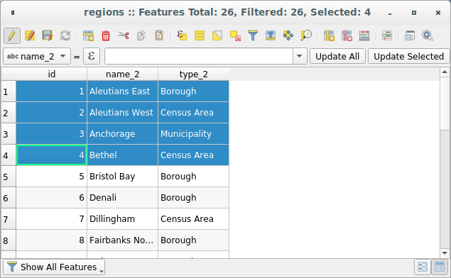
Obr. 16.67 Attribute Table for regions layer
The buttons at the top of the attribute table window provide the following functionality:
Ikona |
Label |
Účel |
Default Shortcut |
|---|---|---|---|
|
Toggle editing mode |
Enable editing functionalities |
Ctrl+E |
|
Toggle multi edit mode |
Update multiple fields of many features |
|
|
Save Edits |
Save current modifications |
|
|
Reload the table |
||
|
Add feature |
Add new geometryless feature |
|
|
Delete selected features |
Remove selected features from the layer |
|
|
Cut selected features to clipboard |
Ctrl+X |
|
|
Copy selected features to clipboard |
Ctrl+C |
|
|
Paste features from clipboard |
Insert new features from copied ones |
Ctrl+V |
|
Select features using an Expression |
||
|
Select All |
Select all features in the layer |
Ctrl+A |
|
Invert selection |
Invert the current selection in the layer |
Ctrl+R |
|
Deselect all |
Deselect all features in the current layer |
Ctrl+Shift+A |
|
Filter/Select features using form |
Ctrl+F |
|
|
Move selected to top |
Move selected rows to the top of the table |
|
|
Pan map to the selected rows |
Ctrl+P |
|
|
Zoom map to the selected rows |
Ctrl+J |
|
|
New field |
Add a new field to the data source |
Ctrl+W |
|
Delete field |
Remove a field from the data source |
|
|
Organize columns |
Show/hide fields from the attribute table |
|
|
Open field calculator |
Update field for many features in a row |
Ctrl+I |
|
Conditional formatting |
Enable table formatting |
|
|
Dock attribute table |
Allows to dock/undock the attribute table |
|
|
Actions |
Lists the actions related to the layer |


Poznámka
Depending on the format of the data and the GDAL library built with your QGIS version, some tools may not be available.
Below these buttons is the Quick Field Calculation bar (enabled only in
edit mode), which allows to quickly apply
calculations to all or part of the features in the layer. This bar uses the same
expressions as the  Field
Calculator (see Editing attribute values).
Field
Calculator (see Editing attribute values).
The attribute table support Shift+Mouse Wheel scrolling in attribute table to switch to a horizontal scrolling action instead of vertical.
16.2.2.1. Table view vs Form view
QGIS provides two view modes to easily manipulate data in the attribute table:
The
Table view, displays values of multiple features in a
tabular mode, each row representing a feature and each column a field.
A right-click on the column header allows you to configure the table
display while a right-click on a cell provides
interaction with the feature.The
 Form view shows feature identifiers in a first panel and displays only the attributes of the clicked
identifier in the second one.
There is a pull-down menu at the top of the first panel where the „identifier“
can be specified using an attribute (Column preview) or an
Expression.
The pull-down also includes the last 10 expressions for re-use.
Form view uses the layer fields configuration
(see Attributes Form Properties).
Form view shows feature identifiers in a first panel and displays only the attributes of the clicked
identifier in the second one.
There is a pull-down menu at the top of the first panel where the „identifier“
can be specified using an attribute (Column preview) or an
Expression.
The pull-down also includes the last 10 expressions for re-use.
Form view uses the layer fields configuration
(see Attributes Form Properties).You can browse through the feature identifiers with the arrows on the bottom of the first panel. The features attributes update in the second panel as you go. It’s also possible to identify or move to the active feature in the map canvas with pushing down any of the button at the bottom:
 Highlight current feature if visible in the
map canvas
Highlight current feature if visible in the
map canvas Automatically pan to current feature
 Zoom to current feature
You can switch from one mode to the other by clicking the corresponding icon at the bottom right of the dialog.
You can also specify the Default view mode at the opening of the attribute table in menu. It can be ‚Remember last view‘, ‚Table view‘ or ‚Form view‘.
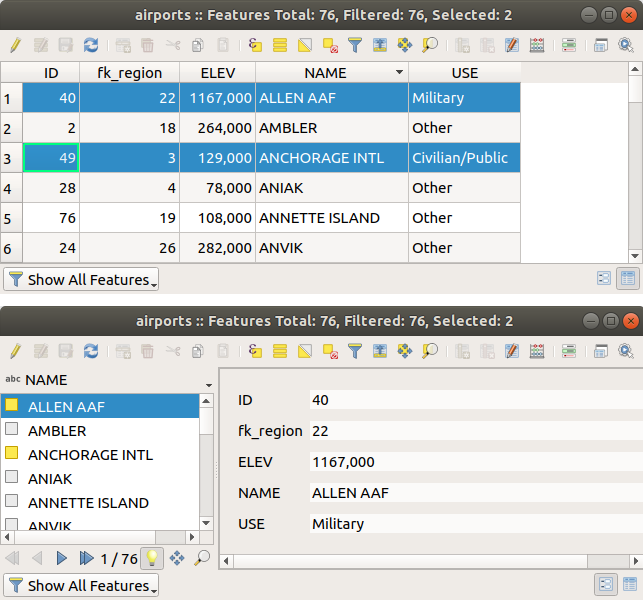
Obr. 16.68 Attribute table in table view (top) vs form view (bottom)
16.2.2.2. Configuring the columns
Right-click in a column header when in table view to have access to tools that help you control:
Resizing columns widths
Columns width can be set through a right-click on the column header and select either:
Set width… to enter the desired value. By default, the current value is displayed in the widget
Set all column widths… to the same value
Autosize to resize at the best fit the column.
Autosize all columns
A column size can also be changed by dragging the boundary on the right of its heading. The new size of the column is maintained for the layer, and restored at the next opening of the attribute table.
Hiding and organizing columns and enabling actions
By right-clicking in a column header, you can choose to Hide column
from the attribute table (in „table view“ mode).
For more advanced controls, press the  Organize columns…
button from the dialog toolbar or choose Organize columns…
in a column header contextual menu.
In the new dialog, you can:
Organize columns…
button from the dialog toolbar or choose Organize columns…
in a column header contextual menu.
In the new dialog, you can:
check/uncheck columns you want to show or hide: a hidden column will disappear from every instances of the attribute table dialog until it is actively restored.
drag-and-drop items to reorder the columns in the attribute table. Note that this change is for the table rendering and does not alter the fields order in the layer datasource
add a new virtual Actions column that displays in each row a drop-down box or a button list of enabled actions. See Actions Properties for more information about actions.
Sorting columns
The table can be sorted by any column, by clicking on the column header. A
small arrow indicates the sort order (downward pointing means descending
values from the top row down, upward pointing means ascending values from
the top row down).
You can also choose to sort the rows with the Sort… option of the
column header context menu and write an expression. E.g. to sort the rows
using multiple columns you can write concat(col0, col1).
In form view, features identifier can be sorted using the  Sort
by preview expression option.
Sort
by preview expression option.
Tip
Sorting based on columns of different types
Trying to sort an attribute table based on columns of string and numeric types
may lead to unexpected result because of the concat("USE", "ID") expression
returning string values (ie, 'Borough105' < 'Borough6').
You can workaround this by using eg concat("USE", lpad("ID", 3, 0)) which
returns 'Borough105' > 'Borough006'.
16.2.2.3. Formatting of table cells using conditions
Conditional formatting settings can be used to highlight in the attribute table features you may want to put a particular focus on, using custom conditions on feature’s:
geometry (e.g., identifying multi-parts features, small area ones or in a defined map extent…);
or field value (e.g., comparing values to a threshold, identifying empty cells…).
You can enable the conditional formatting panel clicking on
 at the top right of the attributes window in table
view (not available in form view).
at the top right of the attributes window in table
view (not available in form view).
The new panel allows user to add new rules to format rendering of
 Field or
  Full row.
Adding new rule opens a form to define:
Full row.
Adding new rule opens a form to define:
the name of the rule;
a condition using any of the expression builder functions;
the formatting: it can be choosen from a list of predefined formats or created based on properties like:
background and text colors;
use of icon;
bold, italic, underline, or strikeout;
font.
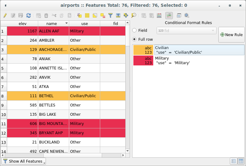
Obr. 16.69 Conditional Formatting of an attribute table
16.2.3. Interacting with features in an attribute table
16.2.3.1. Selecting features
In table view, each row in the attribute table displays the attributes of a unique feature in the layer. Selecting a row selects the feature and likewise, selecting a feature in the map canvas (in case of geometry enabled layer) selects the row in the attribute table. If the set of features selected in the map canvas (or attribute table) is changed, then the selection is also updated in the attribute table (or map canvas) accordingly.
Rows can be selected by clicking on the row number on the left side of the row. Multiple rows can be marked by holding the Ctrl key. A continuous selection can be made by holding the Shift key and clicking on several row headers on the left side of the rows. All rows between the current cursor position and the clicked row are selected. Moving the cursor position in the attribute table, by clicking a cell in the table, does not change the row selection. Changing the selection in the main canvas does not move the cursor position in the attribute table.
In form view of the attribute table, features are by default identified in the left panel by the value of their displayed field (see Display Properties). This identifier can be replaced using the drop-down list at the top of the panel, either by selecting an existing field or using a custom expression. You can also choose to sort the list of features from the drop-down menu.
Click a value in the left panel to display the feature’s attributes in the right one. To select a feature, you need to click inside the square symbol at the left of the identifier. By default, the symbol turns into yellow. Like in the table view, you can perform multiple feature selection using the keyboard combinations previously exposed.
Beyond selecting features with the mouse, you can perform automatic selection based on feature’s attribute using tools available in the attribute table toolbar, such as (see section Automatic selection and following one for more information and use case):
 Select By Expression…
 Select Features By Value…
 Deselect All Features from the Layer
 Select All Features
 Invert Feature Selection.
It is also possible to select features using the Filtering and selecting features using forms.
16.2.3.2. Filtering features
Once you have selected features in the attribute table, you may want to display only these records in the table. This can be easily done using the Show Selected Features item from the drop-down list at the bottom left of the attribute table dialog. This list offers the following filters:
- Show All Features
 Show Selected Features - same as using
Open Attribute Table (Selected Features) from the Layer
menu or the Attributes Toolbar or pressing Shift+F6
Show Selected Features - same as using
Open Attribute Table (Selected Features) from the Layer
menu or the Attributes Toolbar or pressing Shift+F6 Show Features visible on map - same as using
Open Attribute Table (Visible Features) from the Layer
menu or the Attributes Toolbar or pressing Ctrl+F6
Show Features visible on map - same as using
Open Attribute Table (Visible Features) from the Layer
menu or the Attributes Toolbar or pressing Ctrl+F6 Show Edited and New Features - same as using
Open Attribute Table (Edited and New Features) from the Layer
menu or the Attributes Toolbar
Show Edited and New Features - same as using
Open Attribute Table (Edited and New Features) from the Layer
menu or the Attributes ToolbarField Filter - allows the user to filter based on value of a field: choose a column from a list, type or select a value and press Enter to filter. Then, only the features matching
num_field = valueorstring_field ilike '%value%'expression are shown in the attribute table. You can check Case sensitive to be less permissive with strings.
Advanced filter (Expression) - Opens the expression builder dialog. Within it, you can create complex expressions to match table rows. For example, you can filter the table using more than one field. When applied, the filter expression will show up at the bottom of the form.
: a shortcut to saved expressions frequently used for filtering your attribute table.
It is also possible to filter features using forms.
Poznámka
Filtering records out of the attribute table does not filter features out of the layer; they are simply momentaneously hidden from the table and can be accessed from the map canvas or by removing the filter. For filters that do hide features from the layer, use the Query Builder.
Tip
Update datasource filtering with Show Features Visible on Map
When for performance reasons, features shown in attribute table are spatially limited to the canvas extent at its opening (see Data Source Options for a how-to), selecting Show Features Visible on Map on a new canvas extent updates the spatial restriction.
16.2.3.3. Storing filter expressions
Expressions you use for attribute table filtering can be saved for further calls.
When using Field Filter or Advanced Filter (expression)
entries, the expression used is displayed in a text widget in the bottom of the
attribute table dialog. Press the  Save expression with text as name next to the box to save the expression
in the project. Pressing the drop-down menu next to the button allows to save
the expression with a custom name (Save expression as…).
Once a saved expression is displayed, the
Save expression with text as name next to the box to save the expression
in the project. Pressing the drop-down menu next to the button allows to save
the expression with a custom name (Save expression as…).
Once a saved expression is displayed, the  button is triggered and its drop-down menu allows you to Edit the
expression and name if any, or Delete stored expression.
button is triggered and its drop-down menu allows you to Edit the
expression and name if any, or Delete stored expression.
Saved filter expressions are saved in the project and available through the Stored filter expressions menu of the attribute table. They are different from the user expressions, shared by all projects of the active user profile.
16.2.3.4. Filtering and selecting features using forms
Clicking the  Filter/Select features using form or
pressing Ctrl+F will make the attribute table dialog switch to form view
and replace each widget with its search variant.
Filter/Select features using form or
pressing Ctrl+F will make the attribute table dialog switch to form view
and replace each widget with its search variant.
From this point onwards, this tool functionality is similar to the one described in Select Features By Value, where you can find descriptions of all operators and selecting modes.
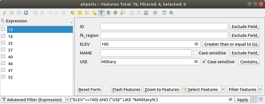
Obr. 16.70 Attribute table filtered by the filter form
When selecting / filtering features from the attribute table, there is a Filter features button that allows defining and refining filters. Its use triggers the Advanced filter (Expression) option and displays the corresponding filter expression in an editable text widget at the bottom of the form.
If there are already filtered features, you can refine the filter using the drop-down list next to the Filter features button. The options are:
Filter within („AND“)
Extend filter („OR“)
To clear the filter, either select the Show all features option from the bottom left pull-down menu, or clear the expression and click Apply or press Enter.
16.2.4. Using action on features
Users have several possibilities to manipulate feature with the contextual menu like:
Select all (Ctrl+A) the features;
Copy the content of a cell in the clipboard with Copy cell content;
Zoom to feature without having to select it beforehand;
Pan to feature without having to select it beforehand;
Flash feature, to highlight it in the map canvas;
Open form: it toggles attribute table into form view with a focus on the clicked feature.
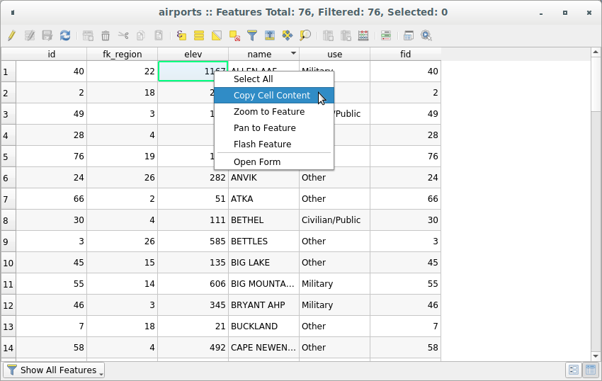
Obr. 16.71 Copy cell content button
If you want to use attribute data in external programs (such as Excel,
LibreOffice, QGIS or a custom web application), select one or more row(s) and
use the  Copy selected rows to clipboard button or press
Ctrl+C.
Copy selected rows to clipboard button or press
Ctrl+C.
In menu you can define the format to paste to with Copy features as dropdown list:
Plain text, no geometry,
Plain text, WKT geometry,
GeoJSON
You can also display a list of actions in this contextual menu. This is enabled in the tab. See Actions Properties for more information on actions.
16.2.4.1. Saving selected features as new layer
The selected features can be saved as any OGR-supported vector format and
also transformed into another coordinate reference system (CRS). In the
contextual menu of the layer, from the Layers panel, click on
to define the name of
the output dataset, its format and CRS (see section Creating new layers from an existing layer). You’ll
notice that is checked.
It is also possible to specify GDAL creation options within the dialog.
16.2.5. Editing attribute values
Editing attribute values can be done by:
typing the new value directly in the cell, whether the attribute table is in table or form view. Changes are hence done cell by cell, feature by feature;
using the field calculator: update in a row a field that may already exist or to be created but for multiple features. It can be used to create virtual fields;
using the quick field calculation bar: same as above but for only existing field;
or using the multi edit mode: update in a row multiple fields for multiple features.
16.2.5.1. Using the Field Calculator
The Field Calculator button in the attribute table
allows you to perform calculations on the basis of existing attribute values or
defined functions, for instance, to calculate length or area of geometry
features. The results can be used to update an existing field, or written
to a new field (that can be a virtual one).
The field calculator is available on any layer that supports edit. When you click on the field calculator icon the dialog opens (see Obr. 16.72). If the layer is not in edit mode, a warning is displayed and using the field calculator will cause the layer to be put in edit mode before the calculation is made.
Based on the Expression Builder dialog, the field calculator dialog offers a complete interface to define an expression and apply it to an existing or a newly created field. To use the field calculator dialog, you must select whether you want to:
apply calculation on the whole layer or on selected features only
create a new field for the calculation or update an existing one.
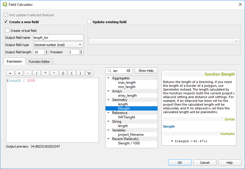
Obr. 16.72 Field Calculator
If you choose to add a new field, you need to enter a field name, a field type (integer, real, date or string) and if needed, the total field length and the field precision. For example, if you choose a field length of 10 and a field precision of 3, it means you have 7 digits before the dot, and 3 digits for the decimal part.
A short example illustrates how field calculator works when using the
Expression tab. We want to calculate the length in km of the
railroads layer from the QGIS sample dataset:
Load the shapefile
railroads.shpin QGIS and press
Open Attribute Table.Click on
 Toggle editing mode and open the
Field Calculator dialog.
Toggle editing mode and open the
Field Calculator dialog.Select the
Create a new field checkbox to save the
calculations into a new field.Set Output field name to
length_kmSelect
Decimal number (real)as Output field typeSet the Output field length to
10and the Precision to3Double click on
$lengthin the Geometry group to add the length of the geometry into the Field calculator expression box (you will begin to see a preview of the output, up to 60 characters, below the expression box updating in real-time as the expression is assembled).Complete the expression by typing
/ 1000in the Field calculator expression box and click OK.You can now find a new length_km field in the attribute table.
16.2.5.2. Creating a Virtual Field
A virtual field is a field based on an expression calculated on the fly, meaning
that its value is automatically updated as soon as an underlying parameter
changes. The expression is set once; you no longer need to recalculate the field
each time underlying values change.
For example, you may want to use a virtual field if you need area to be evaluated
as you digitize features or to automatically calculate a duration between dates
that may change (e.g., using now() function).
Poznámka
Use of Virtual Fields
Virtual fields are not permanent in the layer attributes, meaning that they’re only saved and available in the project file they’ve been created.
A field can be set virtual only at its creation. Virtual fields are marked with a purple background in the fields tab of the layer properties dialog to distinguish them from regular physical or joined fields. Their expression can be edited later by pressing the expression button in the Comment column. An expression editor window will be opened to adjust the expression of the virtual field.
16.2.5.3. Using the Quick Field Calculation Bar
While Field calculator is always available, the quick field calculation bar on top of the attribute table is only visible if the layer is in edit mode. Thanks to the expression engine, it offers a quicker access to edit an already existing field:
Select the field to update in the drop-down list.
Fill the textbox with a value, an expression you directly write or build using the
 expression button.
Click on Update All, Update Selected or Update Filtered button according to your need.
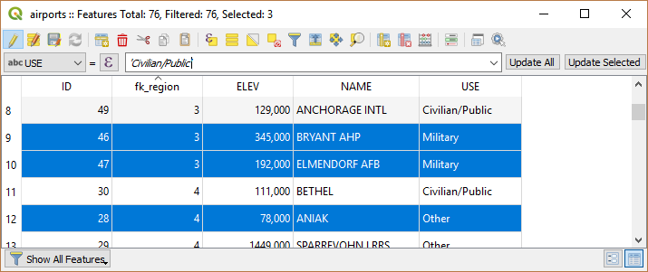
Obr. 16.73 Quick Field Calculation Bar
16.2.5.4. Editing multiple fields
Unlike the previous tools, multi edit mode allows multiple attributes of different features to be edited simultaneously. When the layer is toggled to edit, multi edit capabilities are accessible:
using the
 Toggle multi edit mode button from the toolbar
inside the attribute table dialog;
Toggle multi edit mode button from the toolbar
inside the attribute table dialog;or selecting
menu.
Poznámka
Unlike the tool from the attribute table, hitting the option provides you with a modal dialog to fill attributes changes. Hence, features selection is required before execution.
In order to edit multiple fields in a row:
Select the features you want to edit.
From the attribute table toolbar, click the
button. This will
toggle the dialog to its form view. Feature selection could also be made
at this step.At the right side of the attribute table, fields (and values) of selected features are shown. New widgets appear next to each field allowing for display of the current multi edit state:
 The field contains different values for selected
features. It’s shown empty and each feature will keep its original value.
You can reset the value of the field from the drop-down list of the widget.
The field contains different values for selected
features. It’s shown empty and each feature will keep its original value.
You can reset the value of the field from the drop-down list of the widget. All selected features have the same value for this
field and the value displayed in the form will be kept.
All selected features have the same value for this
field and the value displayed in the form will be kept. The field has been edited and the entered value
will be applied to all the selected features. A message appears at the top
of the dialog, inviting you to either apply or reset your modification.
The field has been edited and the entered value
will be applied to all the selected features. A message appears at the top
of the dialog, inviting you to either apply or reset your modification.
Clicking any of these widgets allows you to either set the current value for the field or reset to original value, meaning that you can roll back changes on a field-by-field basis.
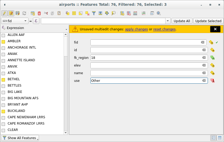
Obr. 16.74 Editing fields of multiple features
Make the changes to the fields you want.
Click on Apply changes in the upper message text or any other feature in the left panel.
Changes will apply to all selected features. If no feature is selected, the
whole table is updated with your changes. Modifications are made as a single
edit command. So pressing  Undo will rollback the attribute
changes for all selected features at once.
Undo will rollback the attribute
changes for all selected features at once.
Poznámka
Multi edit mode is only available for auto generated and drag and drop forms (see Customizing a form for your data); it is not supported by custom ui forms.
16.2.6. Creating one or many to many relations
Relations are a technique often used in databases. The concept is that features (rows) of different layers (tables) can belong to each other.
16.2.6.1. Introducing 1-N relations
As an example you have a layer with all regions of alaska (polygon) which provides some attributes about its name and region type and a unique id (which acts as primary key).
Then you get another point layer or table with information about airports that are located in the regions and you also want to keep track of these. If you want to add them to the regions layer, you need to create a one to many relation using foreign keys, because there are several airports in most regions.
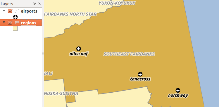
Obr. 16.75 Alaska region with airports
Layers in 1-N relations
QGIS makes no difference between a table and a vector layer. Basically, a vector
layer is a table with a geometry. So you can add your table as a vector layer.
To demonstrate the 1-n relation, you can load the regions shapefile and
the airports shapefile which has a foreign key field (fk_region) to
the layer regions. This means, that each airport belongs to exactly one region
while each region can have any number of airports (a typical one to many
relation).
Foreign keys in 1-N relations
In addition to the already existing attributes in the airports attribute table,
you’ll need another field fk_region which acts as a foreign key (if you have
a database, you will probably want to define a constraint on it).
This field fk_region will always contain an id of a region. It can be seen like a pointer to the region it belongs to. And you can design a custom edit form for editing and QGIS takes care of the setup. It works with different providers (so you can also use it with shape and csv files) and all you have to do is to tell QGIS the relations between your tables.
Defining 1-N relations
The first thing we are going to do is to let QGIS know about the relations
between the layers. This is done in .
Open the Relations tab and click on  Add Relation.
Name is going to be used as a title. It should be a human readable string, describing, what the relation is used for. We will just call say airport_relation in this case.
Referenced Layer (Parent) also considered as parent layer, is the one with the primary key, pointed to, so here it is the
regionslayer. You need to define the primary key of the referenced layer, so it isID.Referencing Layer (Child) also considered as child layer, is the one with the foreign key field on it. In our case, this is the
airportslayer. For this layer you need to add a referencing field which points to the other layer, so this isfk_region.Poznámka
Sometimes, you need more than a single field to uniquely identify features in a layer. Creating a relation with such a layer requires a composite key, ie more than a single pair of matching fields. Use the
Add new field pair as part of a composite
foreign key button to add as many pairs as necessary.Id will be used for internal purposes and has to be unique. You may need it to build custom forms. If you leave it empty, one will be generated for you but you can assign one yourself to get one that is easier to handle
Relationship strength sets the strength of the relation between the parent and the child layer. The default Association type means that the parent layer is simply linked to the child one while the Composition type allows you to duplicate also the child features when duplicating the parent ones and on deleting a feature the children are deleted as well, resulting in cascade over all levels (means children of children of… are deleted as well).
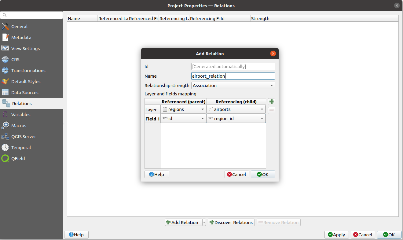
Obr. 16.76 Adding a relation between regions and airports layers
From the Relations tab, you can also press the
Discover Relation button to fetch the relations available from
the providers of the loaded layers. This is possible for layers stored in
data providers like PostgreSQL or SpatiaLite.
Forms for 1-N relations
Now that QGIS knows about the relation, it will be used to improve the forms it generates. As we did not change the default form method (autogenerated) it will just add a new widget in our form. So let’s select the layer region in the legend and use the identify tool. Depending on your settings, the form might open directly or you will have to choose to open it in the identification dialog under actions.
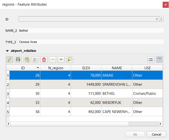
Obr. 16.77 Identification dialog regions with relation to airports
As you can see, the airports assigned to this particular region are all shown in a table. And there are also some buttons available. Let’s review them shortly:
The
button is for toggling the edit mode. Be aware that it
toggles the edit mode of the airport layer, although we are in the feature
form of a feature from the region layer. But the table is representing
features of the airport layer.The
 button is for saving all the edits in the child layer (airport).
The
 button lets you digitize the airport geometry in the map canvas and
assigns the new feature to the current region by default.
Note that the icon will change according to the geometry type.
button lets you digitize the airport geometry in the map canvas and
assigns the new feature to the current region by default.
Note that the icon will change according to the geometry type.The
 button adds a new record to the airport layer attribute table
and assigns the new feature to the current region by default. The geometry can
be drawn later with the Add part digitizing tool.
button adds a new record to the airport layer attribute table
and assigns the new feature to the current region by default. The geometry can
be drawn later with the Add part digitizing tool.The
 button allows you to copy and paste one or more child
features within the child layer. They can later be assigned to a different
parent feature or have their attributes modified.
button allows you to copy and paste one or more child
features within the child layer. They can later be assigned to a different
parent feature or have their attributes modified.The
 button deletes the selected airport(s) permanently.
The
 symbol opens a new dialog where you can select any existing
airport which will then be assigned to the current region. This may be handy
if you created the airport on the wrong region by accident.
symbol opens a new dialog where you can select any existing
airport which will then be assigned to the current region. This may be handy
if you created the airport on the wrong region by accident.The
 symbol unlinks the selected airport(s) from the current region,
leaving them unassigned (the foreign key is set to NULL) effectively.
symbol unlinks the selected airport(s) from the current region,
leaving them unassigned (the foreign key is set to NULL) effectively.With the
 button you can zoom the map to the selected child
features.
button you can zoom the map to the selected child
features.The two buttons
and to the right switch between the table
view and form view of the related child features.
If you use the Drag and Drop Designer for the regions feature, you can select which tools are available. You can even decide whether to open a new form when a new feature is added using Force hide form on add feature option. Be aware that this option implies that not null attributes must take a valid default value to work correctly.
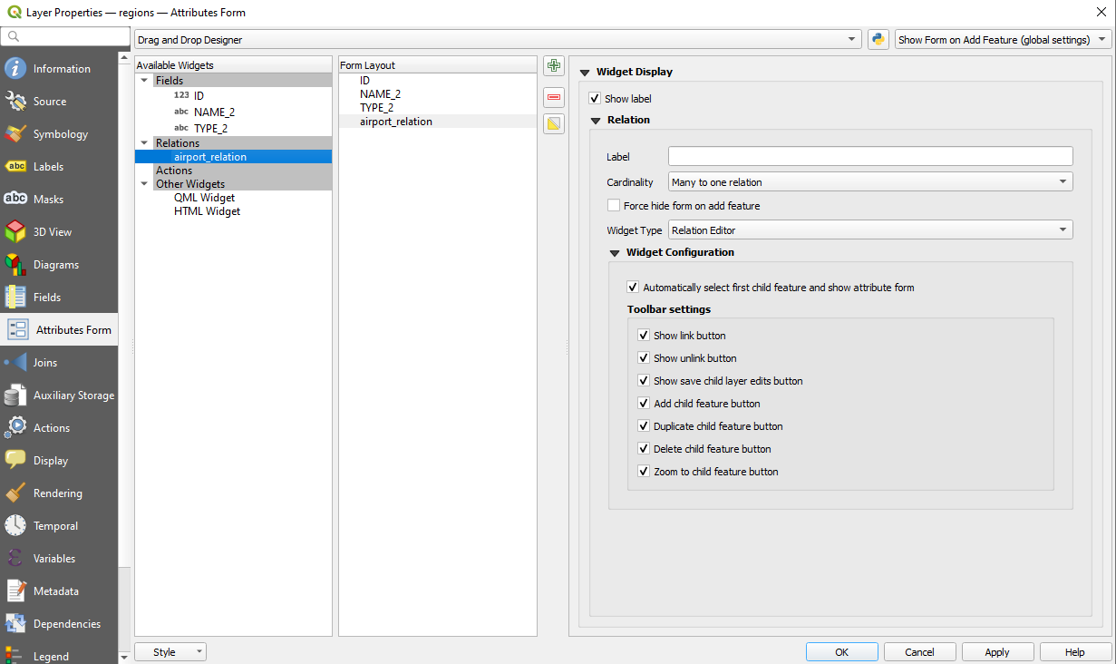
Obr. 16.78 Drag and Drop Designer for configure regions-airports relation tools
In the above example the referencing layer has geometries (so it isn’t just an alphanumeric table) so the above steps will create an entry in the layer attribute table that has no corresponding geometric feature. To add the geometry:
Choose
for the referencing layer.Select the record that has been added previously within the feature form of the referenced layer.
Use the
 Add Part digitizing tool to attach a geometry to the
selected attributes table record.
Add Part digitizing tool to attach a geometry to the
selected attributes table record.
If you work on the airport table, the widget Relation Reference is automatically
set up for the fk_region field (the one used to create the relation), see
Relation Reference widget.
In the airport form you will see the button at the right side of the
fk_region field: if you click on the button the form of the region layer will
be opened. This widget allows you to easily and quickly open the forms of the
linked parent features.
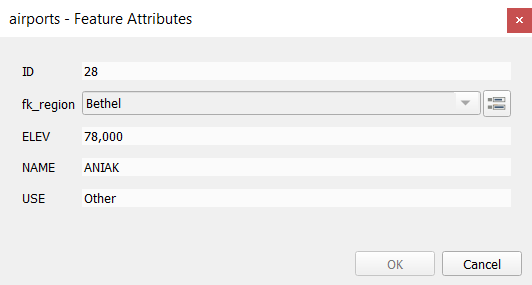
Obr. 16.79 Identification dialog airport with relation to regions
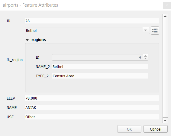
The Relation Reference widget has also an option to embed the form of the parent
layer within the child one. It is available in the
menu of the airport layer: select the fk_region field and check the
Show embedded form option.
If you look at the feature dialog now, you will see, that the form of the region is embedded inside the airports form and will even have a combobox, which allows you to assign the current airport to another region.
Moreover if you toggle the editing mode of the airport layer, the fk_region
field has also an autocompleter function: while typing you will see all the
values of the id field of the region layer.
Here it is possible to digitize a polygon for the region layer using the button
if you chose the option Allow adding new features in the
menu of the airport layer.
The child layer can also be used in the Select Features By Value tool in order to select features of the parent layer based on attributes of their children.
In Obr. 16.80, all the regions where the mean altitude of the airports is greater than 500 meters above sea level are selected.
You will find that many different aggregation functions are available in the form.
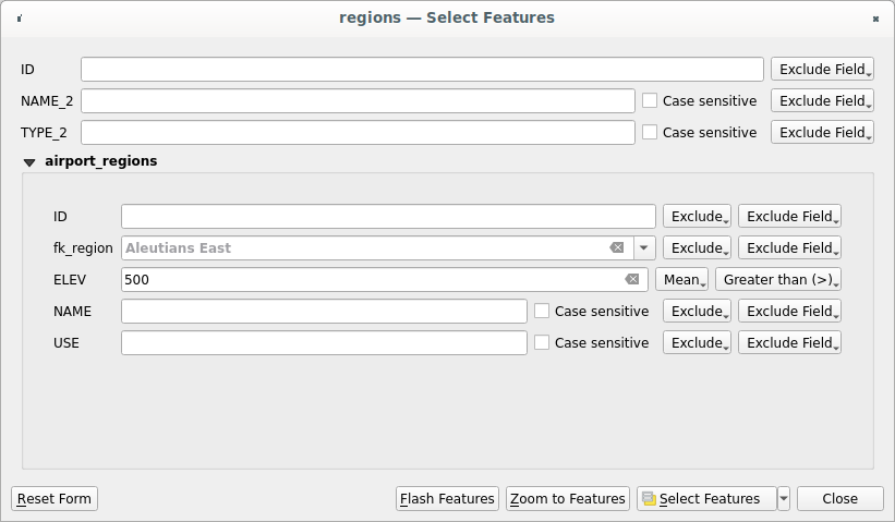
Obr. 16.80 Select parent features with child values
16.2.6.2. Introducing many-to-many (N-M) relations
N-M relations are many-to-many relations between two tables. For instance, the
airports and airlines layers: an airport receives several airline
companies and an airline company flies to several airports.
This SQL code creates the three tables we need for an N-M relationship in
a PostgreSQL/PostGIS schema named locations. You can run the code using the
for PostGIS or external tools such as pgAdmin. The airports table stores the airports layer and the airlines
table stores the airlines layer. In both tables few fields are used for
clarity. The tricky part is the airports_airlines table. We need it to list all
airlines for all airports (or vice versa). This kind of table is known
as a pivot table. The constraints in this table force that an airport can be
associated with an airline only if both already exist in their layers.
CREATE SCHEMA locations;

CREATE TABLE locations.airports
(
   id serial NOT NULL,
   geom geometry(Point, 4326) NOT NULL,
   airport_name text NOT NULL,
   CONSTRAINT airports_pkey PRIMARY KEY (id)
);

CREATE INDEX airports_geom_idx ON locations.airports USING gist (geom);

CREATE TABLE locations.airlines
(
   id serial NOT NULL,
   geom geometry(Point, 4326) NOT NULL,
   airline_name text NOT NULL,
   CONSTRAINT airlines_pkey PRIMARY KEY (id)
);

CREATE INDEX airlines_geom_idx ON locations.airlines USING gist (geom);

CREATE TABLE locations.airports_airlines
(
   id serial NOT NULL,
   airport_fk integer NOT NULL,
   airline_fk integer NOT NULL,
   CONSTRAINT airports_airlines_pkey PRIMARY KEY (id),
   CONSTRAINT airports_airlines_airport_fk_fkey FOREIGN KEY (airport_fk)
      REFERENCES locations.airports (id)
      ON DELETE CASCADE
      ON UPDATE CASCADE
      DEFERRABLE INITIALLY DEFERRED,
   CONSTRAINT airports_airlines_airline_fk_fkey FOREIGN KEY (airline_fk)
      REFERENCES locations.airlines (id)
      ON DELETE CASCADE
      ON UPDATE CASCADE
      DEFERRABLE INITIALLY DEFERRED
 );
Instead of PostgreSQL you can also use GeoPackage. In this case, the three tables can be created manually using the . In GeoPackage there are no schemas so the locations prefix is not needed.
Foreign key constraints in airports_airlines table can´t be created using
or
so they should be created using .
GeoPackage doesn’t support ADD CONSTRAINT statements so the airports_airlines
table should be created in two steps:
Set up the table only with the
idfield usingUsing , type and execute this SQL code:
ALTER TABLE airports_airlines
   ADD COLUMN airport_fk INTEGER
   REFERENCES airports (id)
   ON DELETE CASCADE
   ON UPDATE CASCADE
   DEFERRABLE INITIALLY DEFERRED;

ALTER TABLE airports_airlines
   ADD COLUMN airline_fk INTEGER
   REFERENCES airlines (id)
   ON DELETE CASCADE
   ON UPDATE CASCADE
   DEFERRABLE INITIALLY DEFERRED;
Then in QGIS, you should set up two one-to-many relations as explained above:
a relation between
airlinestable and the pivot table;and a second one between
airportstable and the pivot table.
An easier way to do it (only for PostgreSQL) is using the Discover Relations in . QGIS will automatically read all relations in your database and you only have to select the two you need. Remember to load the three tables in the QGIS project first.
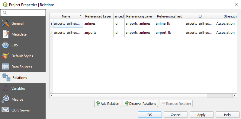
Obr. 16.81 Relations and autodiscover
In case you want to remove an airport or an airline, QGIS won’t remove
the associated record(s) in airports_airlines table. This task will be made by
the database if we specify the right constraints in the pivot table creation as
in the current example.
Poznámka
Combining N-M relation with automatic transaction group
You should enable the transaction mode in when working on such context. QGIS should be able to add or update row(s) in all tables (airlines, airports and the pivot tables).
Finally we have to select the right cardinality in the
for the airports and
airlines layers. For the first one we should choose the airlines (id) option
and for the second one the airports (id) option.
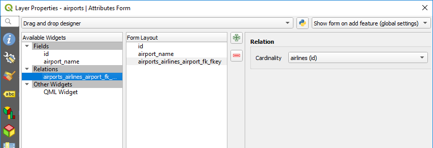
Obr. 16.82 Set relationship cardinality
Now you can associate an airport with an airline (or an airline with an airport)
using Add child feature or Link existing child feature
in the subforms. A record will automatically be inserted in the airports_airlines
table.
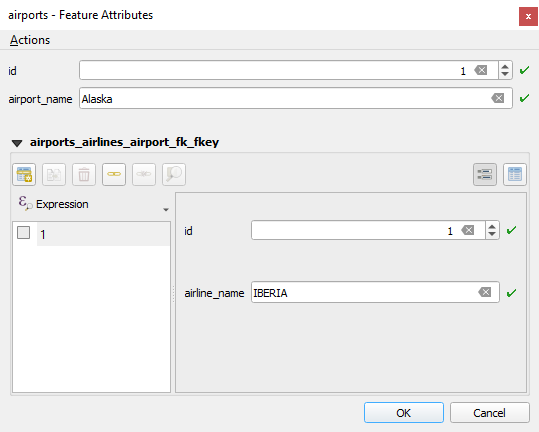
Obr. 16.83 N-M relationship between airports and airlines
Poznámka
Using Many to one relation cardinality
Sometimes hiding the pivot table in an N-M relationship is not desirable. Mainly because there are attributes in the relationship that can only have values when a relationship is established. If your tables are layers (have a geometry field) it could be interesting to activate the On map identification option () for the foreign key fields in the pivot table.
Poznámka
Pivot table primary key
Avoid using multiple fields in the primary key in a pivot table. QGIS assumes a single
primary key so a constraint like constraint airports_airlines_pkey primary key (airport_fk, airline_fk)
will not work.
16.2.6.3. Introducing polymorphic relations
Polymorphic relations are special case of 1-N relations, where a single referencing (document) layer contains
the features for multiple referenced layers. This differs from normal relations which require different
referencing layer for each referenced layer. A single referencing (document) layer is achieved by adding an adiditonal
layer_field column in the referencing (document) layer that stores information to identify the referenced layer. In
its most simple form, the referencing (document) layer will just insert the layer name of the referenced layer into
this field.
To be more precise, a polymorphic relation is a set of normal relations having the same referencing layer but having the referenced layer dynamically defined. The polymorphic setting of the layer is solved by using an expression which has to match some properties of the referenced layer like the table name, layer id, layer name.
Imagine we are going to the park and want to take pictures of different species of plants and animals
we see there. Each plant or animal has multiple pictures associated with it, so if we use the normal 1:N
relations to store pictures, we would need two separate tables, animal_images and plant_images.
This might not be a problem for 2 tables, but imagine if we want to take separate pictures for mushrooms, birds etc.
Polymorphic relations solve this problem as all the referencing features are stored in the same table documents.
For each feature the referenced layer is stored in the referenced_layer field and the referenced
feature id in the referenced_fk field.
Defining polymorphic relations
First, let QGIS know about the polymorphic relations between the layers. This is
done in .
Open the Relations tab and click on the little down arrow next to the
Add Relation button, so you can select the Add Polymorphic Relation option
from the newly appeared dropdown.
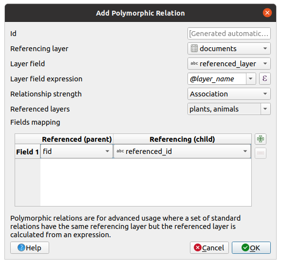
Obr. 16.84 Adding a polymorphic relation using documents layer as referencing and animals and plants as referenced layers.
Id will be used for internal purposes and has to be unique. You may need it to build custom forms. If you leave it empty, one will be generated for you but you can assign one yourself to get one that is easier to handle
Referencing Layer (Child) also considered as child layer, is the one with the foreign key field on it. In our case, this is the
documentslayer. For this layer you need to add a referencing field which points to the other layer, so this isreferenced_fk.Poznámka
Sometimes, you need more than a single field to uniquely identify features in a layer. Creating a relation with such a layer requires a composite key, ie more than a single pair of matching fields. Use the
Add new field pair as part of a composite
foreign key button to add as many pairs as necessary.Layer Field is the field in the referencing table that stores the result of the evaluated layer expression which is the referencing table that this feature belongs to. In our example, this would be the
referenced_layerfield.Layer expression evaluates to a unique identifier of the layer. This can be the layer name
@layer_name, the layer id@layer_id, the layer’s table namedecode_uri(@layer, 'table')or anything that can uniquely identifies a layer.Relationship strength sets the strength of the generated relations between the parent and the child layer. The default Association type means that the parent layer is simply linked to the child one while the Composition type allows you to duplicate also the child features when duplicating the parent ones and on deleting a feature the children are deleted as well, resulting in cascade over all levels (means children of children of… are deleted as well).
Referenced Layers also considered as parent layers, are those with the primary key, pointed to, so here they would be
plantsandanimalslayers. You need to define the primary key of the referenced layers from the dropdown, so it isfid. Note that the definition of a valid primary key requires all the referenced layers to have a field with that name. If there is no such field you cannot save a polymorphic relation.
Once added, the polymorphic relation can be edited via the Edit Polymorphic Relation menu entry.
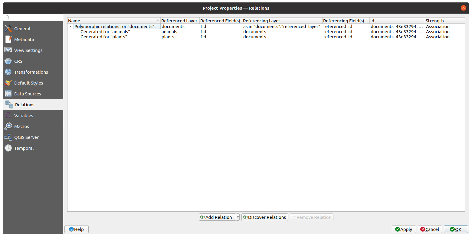
Obr. 16.85 Preview of the newly created polymorphic relation and it’s child relations for animals and plants.
The example above uses the following database schema:
CREATE SCHEMA park;

CREATE TABLE park.animals
(
   fid serial NOT NULL,
   geom geometry(Point, 4326) NOT NULL,
   animal_species text NOT NULL,
   CONSTRAINT animals_pkey PRIMARY KEY (fid)
);

CREATE INDEX animals_geom_idx ON park.animals USING gist (geom);

CREATE TABLE park.plants
(
   fid serial NOT NULL,
   geom geometry(Point, 4326) NOT NULL,
   plant_species text NOT NULL,
   CONSTRAINT plants_pkey PRIMARY KEY (fid)
);

CREATE INDEX plants_geom_idx ON park.plants USING gist (geom);

CREATE TABLE park.documents
(
   fid serial NOT NULL,
   referenced_layer text NOT NULL,
   referenced_fk integer NOT NULL,
   image_filename text NOT NULL,
   CONSTRAINT documents_pkey PRIMARY KEY (fid)
);
16.2.7. Storing and fetching an external resource
A field may target a resource stored on an external storage system. Attribute forms can be configured so they act as a client to an external storage system in order to store and fetch those resources, on users demand, directly from the forms.
16.2.7.1. Configuring an external storage
In order to setup an external storage, you have to first configure it from the vector attribute form properties and select the Attachment widget.
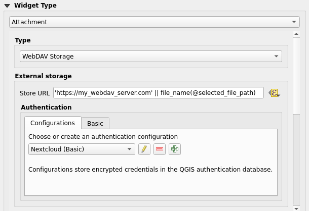
Obr. 16.86 Editing a WebDAV external storage for a given field
From the Attachment widget, you have to first select the Storage type:
Select Existing File: The target URL already exists. When you select a resource, no store operation is achieved, the attribute is simply updated with the URL.
Simple Copy: Stores a copy of the resource on a file disk destination (which could be a local or network shared file system) and the attribute is updated with the path to the copy.
WebDAV Storage: The resource is pushed to a HTTP server supporting the WebDAV protocol and the attribute is updated with its URL. Nextcloud, Pydio or other file hosting software support this protocol.
Then, you have to set up the Store URL parameter, which provides the URL to be used when a new resource needs to be stored. It’s possible to set up an expression using the data defined override widget in order to have specific values according to feature attributes.
The variable @selected_file_path could be used in that expression and represent the absolute file path of the user selected file (using the file selector or drag’n drop).
Poznámka
Using the WebDAV external storage, if the URL ends with a „/“, it is considered as a folder and the selected file name will be appended to get the final URL.
If the external storage system needs to, it’s possible to configure an authentication.
16.2.7.2. Using an external storage
Once configured, you can select a local file using the button … when editing a feature’s attribute. Depending on the configured storage type, the file will be stored on the external storage system (except if Select existing file has been selected) and the field will be updated with the new resource URL.
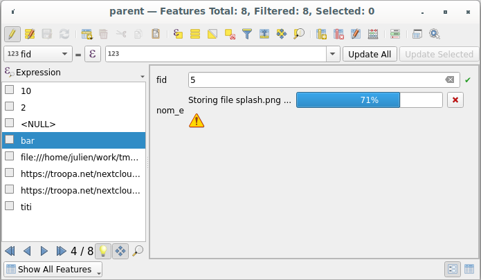
Obr. 16.87 Storing a file to a WebDAV external storage
Poznámka
User can also achieve the same result if he drags and drops a file on the whole attachment widget.
Use the  Cancel button to abort the storing process.
It’s possible to configure a viewer using the Integrated document viewer
so the resource will be automatically fetched from the external storage system and
displayed directly below the URL.
The above
Cancel button to abort the storing process.
It’s possible to configure a viewer using the Integrated document viewer
so the resource will be automatically fetched from the external storage system and
displayed directly below the URL.
The above  icon indicates that the resource cannot be fetched
from the external storage system. In that case, more details might appear in the
Log Messages Panel.
icon indicates that the resource cannot be fetched
from the external storage system. In that case, more details might appear in the
Log Messages Panel.