14.4. Lesson: Updating Forest Stands
Now that you have digitized the information from the old inventory maps and added the corresponding information to the forest stands, the next step would be to create the inventory of the current state of the forest.
You will digitize new forest stands from scratch following an aerial photo from that forest area. The forestry map you digitized in the previous lesson was created from an aerial Color Infrared (CIR) photograph. This type of imagery, where the infrared light is recorded instead of the blue light, are widely used to study vegetated areas. You will also use a CIR photograph in this lesson.
After digitizing the forest stands, you will add information such as new constraints given by conservation regulations.
The goal for this lesson: To digitize a new set of forest stands from CIR aerial photographs and add information from other data-sets.
14.4.1.  Comparing the Old Forest Stands to Current Aerial Photographs
The National Land Survey of Finland has an open data policy that allows you downloading a variety of geographical data like aerial imagery, traditional topographic maps, DEM, LiDAR data, etc. The service can be accessed also in English here. The aerial image used in this exercise has been created from two orthorectified CIR images downloaded from that service (M4134F_21062012 and M4143E_21062012).
Open QGIS and set the project’s CRS to ETRS89 / ETRS-TM35FIN in .
From the
exercise_data\forestry\folder, add the CIR imagerautjarvi_aerial.tifthat is containing the digitized lakes.Then save the QGIS project as
digitizing_2012.qgs.
The CIR images are from 2012. You can compare the stands that were created in 1994 with the situation almost 20 years later.
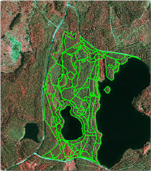
Add your forest_stands_1994.shp layer.
Set its styling so that you can see through your polygons.
Review how the old forest stands follow (or not) what you might visually interpret as an homogeneous forest.
Zoom and pan around the area. You probably will notice that some of the old forest stands might be still corresponding with the image but others are not.
This is a normal situation, as some 20 years have passed by and different forest operations have been done (harvesting, thinning…). It is also possible that the forest stands looked homogeneous back in 1992 to the person who digitized them but as time has passed some forest has developed in different ways. Or simply the priorities for the forest inventory were different that they are today.
Next, you will create new forest stands for this image without using the old ones. Later you can compare them to see the differences.
14.4.2. Interpreting the CIR Image
Let’s digitize the same area that was covered by the old inventory, limited by the roads and the lake. You don’t have to digitize the whole area, as in the previous exercise you can start with a vector file that already contains most of the forest stands.
Remove the forest_stands_1994.shp layer.
Add the forest_stands_2012.shp layer, located in the exercise_data\forestry\ folder.
Set the styling of this layer so that the polygons have no fill and the borders are visible.
You can see that a region to the North of the inventory area is still missing. That will be your task, digitizing the missing forest stands.
But before you start, spend some time reviewing the forest stands already digitized and the corresponding forest in the image. Try to get an idea about how the stands borders are decided, it helps if you have some forestry knowledge.
Some ideas about what you could identify from the images:
What forests are deciduous species (in Finland mostly birch forests) and which ones are conifers (in this region pine or spruce). In CIR images, deciduous species will often come as bright red color whereas conifers present dark green colors.
When a forest stand age changes, by looking at the sizes of the tree crowns that can be identified in the imagery.
The different forest stands’ densities, for example forest stand were a thinning operation has recently been done would clearly show spaces between the tree crowns and should be easy to differentiate from other forest stands around it.
Blueish areas indicate barren terrain, roads and urban areas, crops that have not started to grow etc.
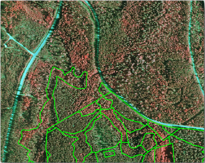
Don’t use zooms too close to the image when trying to identify forest stands. A scale between 1:3 000 and 1: 5 000 should be enough for this imagery. See the image below (1:4000 scale):
14.4.3. Try Yourself Digitizing Forest Stands from CIR Imagery
When digitizing the forest stands, you should try to get forest areas that are as homogeneous as possible in terms of tree species, forest age, stand density… Don’t be too detailed though, or you will end up making hundreds of small forest stands that would not be useful at all. You should try to get stands that are meaningful in the context of forestry, not too small (at least 0.5 ha) but not too big either (no more than 3 ha).
With this indications in mind, you can now digitize the missing forest stands.
Enable editing for forest_stands_2012.shp.
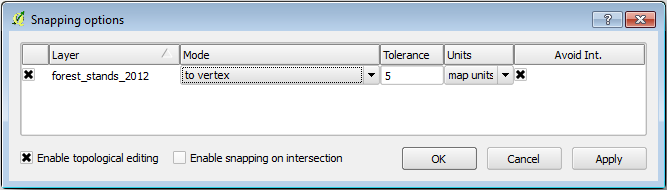
Set up the snapping and topology options as in the image.
Remember to click Apply or OK.
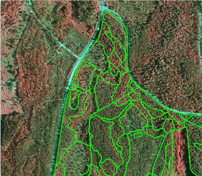
Start digitizing as you did in the previous lesson, with the only difference that you don’t have any point layer that you are snapping to. For this area you should get around 14 new forest stands. While digitizing, fill in the Stand_id field with numbers starting at 901.
When you are finished your layer should look something like:
Now you have a new set of polygons defining the different forest stands for the current situation as can interpreted from the CIR images. But you are obviously still missing the forest inventory data, right? For that you will still need to visit the forest and get some sample data that you will use to estimate the forest attributes for each of the forest stands. You will see how to do that in the next lesson.
For the moment, you still can improve your vector layer with some extra information that you have about conservation regulation that should be taken into account for this area.
14.4.4. Follow Along: Updating Forest Stands with Conservation Information
For the area you are working with, it has been researched that the following conservation regulations must be taken into account while doing the forest planning:
Two locations of a protected species of Siberian flying squirrel (Pteromys volans) have been identified. According to the regulation, an area of 15 meters around the spots must be left untouched.
A riparian forest of special interest growing along a stream in the area must be protected. In a visit to the field, it was found that 20 meters to both sides of the stream must be protected.
You have one vector file containing the information about the squirrel locations and another containing the digitized stream running in the North area towards the lake. From the exercise_data\forestry\ folder, add the vector files squirrel.shp and stream.shp.
For the protection of the squirrels locations, you are going to add a new attribute (column) to your new forest stands that will contain information about point locations that have to be protected. That information will later be available whenever a forest operation is planned, and the field team will be able to mark the area that has to be left untouched before the work starts.
Open the attribute table for the squirrel layer.
You can see that there are two locations that are defined as Siberian flying squirrel, and that the area to be protected is indicated by a distance of 15 meters from the locations.
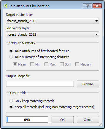
To join the information about the squirrels to your forest stands, you can use the Join attributes by location:
Open .
Set the forest_stands_2012.shp layer as the Target vector layer.
As Join vector layer select the squirrel.shp point layer.
Name the output file as stands_squirrel.shp.
In Output table select Keep all records (including non-matching target records). So that you keep all the forest stands in the layer instead of only keeping those that are spatially related to the squirrel locations.
Click OK.
Select Yes when prompted to add the layer to the TOC.
Close the dialogue box.
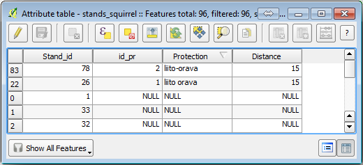
Now you have a new forest stands layer, stands_squirrel where there are new attributes corresponding to the protection information related to the Siberian flying squirrel.
Open the table of the new layer and order it so that the forest stands with information for the Protection attribute are on top. You should have now two forest stands where the squirrel has been located:
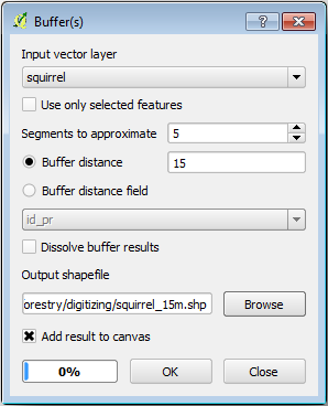
Although this information might be enough, look at what areas related to the squirrels should be protected. You know that you have to leave a buffer of 15 meters around the squirrels location:
Open .
Make a buffer of 15 meters for the squirrel layer.
Name the result squirrel_15m.shp.
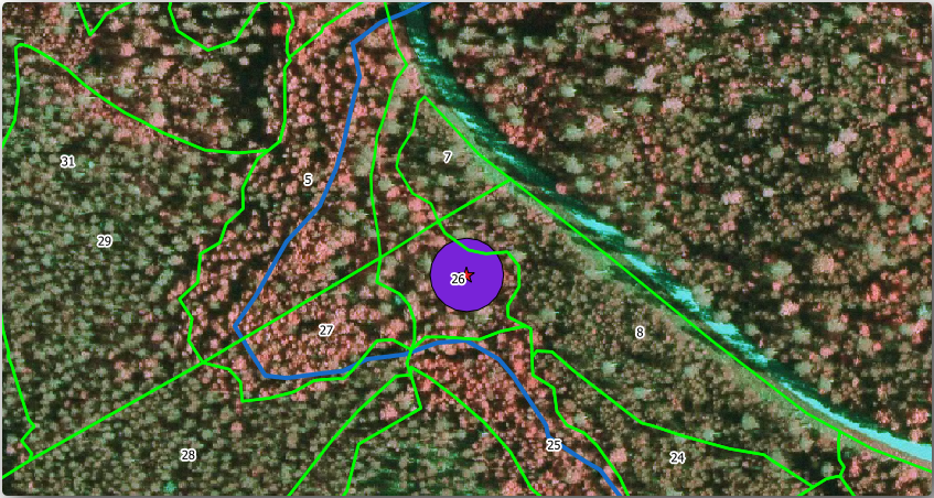
You will notice that if you zoom in to the location in the Northern part of the area, the buffer area extends to the neighbouring stand as well. This means that whenever a forest operation would take place in that stand, the protected location should also be taken into account.
From your previous analysis, you did not get that stand to register information about the protection status. To solve this problem:
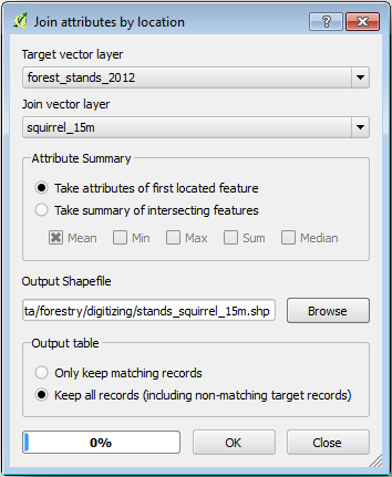
Run the Join attributes by location tool again.
But this time use the squirrel_15m layer as join layer.
Name the output file as stands_squirrel_15m.shp.
Open the attribute table for the this new layer and note that now you have three forest stands that have the information about the protection locations. The information in the forest stands data will indicate to the forest manager that there are protection considerations to be taken into account. Then he or she can get the location from the squirrel dataset, and visit the area to mark the corresponding buffer around the location so that the operators in the field can avoid disturbing the squirrels environment.
14.4.5. Try Yourself Updating Forest Stands with Distance to the Stream
Following the same approach as indicated for the protected squirrel locations you can now update your forest stands with protection information related to the stream identified in the field:
Remember that the buffer in this case is 20 meters around it.
You want to have all the protection information in the same vector file, so use the stands_squirrel_15m layer as the target.
Name your output as forest_stands_2012_protect.shp.
Open the attributes table for the new vector layer and confirm that you now have all the protection information for the stands that are affected by the protection measures to protect the riparian forest associated with the stream.
Save your QGIS project.
14.4.6. In Conclusion
You have seen how to interpret CIR images to digitize forest stands. Of course it would take some practice to make more accurate stands and usually using other information like soil maps would give better results, but you know now the basis for this type of task. And adding information from other datasets resulted to be quite a trivial task.
14.4.7. What’s Next?
The forest stands you digitized will be used for planning forestry operations in the future, but you still need to get more information about the forest. In the next lesson, you will see how to plan a set of sampling plots to inventory the forest area you just digitized, and get the overall estimate of forest parameters.