14.7. Lesson: Calculating the Forest Parameters
Estimating the parameters of the forest is the goal of the forest inventory. Continuing the example from previous lesson, you will use the inventory information gathered in the field to calculate the forest parameters, for the whole forest first, and then for the stands you digitized before.
The goal for this lesson: Calculate forest parameters at general and stand level.
14.7.1.  Follow Along: Adding the Inventory Results
The field teams visited the forest and with the help of the information you provided, gathered information about the forest at every sample plot.
Most often the information will be collected into paper forms in the field,
then typed to a spreadsheet. The sample plots information has been condensed
into a .csv file that can be easily open in QGIS.
Continue with the QGIS project from the lesson about designing the inventory,
you probably named it forest_inventory.qgs.
First, add the sample plots measurements to your QGIS project:
Go to .
Browse to the file
systematic_inventory_results.csvlocated inexercise_data/forestry/results/.Make sure that the Point coordinates option is checked.
Set the fields for the coordinates to the X and Y fields.
Kliknout OK.
When prompted, select ETRS89 / ETRS-TM35FIN as the CRS.
Open the new layer’s Attribute table and have a look at the data.
You can read the type of data that is contained in the sample plots measurements
in the text file legend_2012_inventorydata.txt located in the
exercise_data/forestry/results/ folder.
The systematic_inventory_results layer you just added is actually just
a virtual representation of the text information in the .csv file.
Before you continue, convert the inventory results to a real spatial dataset:
Right click on the
systematic_inventory_resultslayer.Browse to
exercise_data/forestry/results/folder.Name the file
sample_plots_results.shp.Check Add saved file to map.
Remove the
systematic_inventory_resultslayer from your project.
14.7.2. Follow Along: Whole Forest Parameters Estimation
You can calculate the averages for this whole forest area from the inventory
results for the some interesting parameters, like the volume and the number
of stems per hectare. Since the systematic sample plots represent equal areas,
you can directly calculate the averages of the volumes and number of stems per
hectare from the sample_plots_results layer.
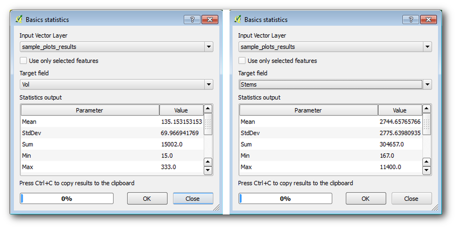
You can calculate the average of a field in a vector layer using the Basic statistics tool:
Open .
Select
sample_plots_resultsas the Input Vector Layer.Select
Volas Target field.Kliknout OK.
The average volume in the forest is 135.2 m3/ha.
You can calculate the average for the number of stems in the same way, 2745 stems/ha.
14.7.3. Follow Along: Estimating Stand Parameters
You can make use of those same systematic sample plots to calculate estimates for the different forest stands you digitized previously. Some of the forest stands did not get any sample plot and for those you will not get information. You could have planned some extra sample plots when you planned the systematic inventory, so that the field teams would have measured a few extra sample plots for this purpose. Or you could send a field team later to get estimates of the missing forest stands to complete the stand inventory. Nevertheless, you will get information for a good number of stands just using the planned plots.
What you need is to get the averages of the sample plots that are falling within each of the forest stands. When you want to combine information based on their relative locations, you perform a spatial join:
Open the tool.
Set
forest_stands_2012as the Target vector layer. The layer you want the results for.Set
sample_plots_resultsas the Join vector layer. The layer you want to calculate estimates from.Check Take summary of intersecting features.
Check to calculate only the Mean.
Name the result as
forest_stands_2012_results.shpand save it in theexercise_data/forestry/results/folder.Finally select Keep all records…, so you can check later what stands did not get information.
Kliknout OK.
Accept adding the new layer to your project when prompted.
Close the Join attributes by location tool.
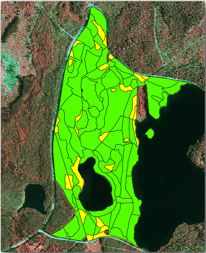
Open the Attribute table for forest_stands_2012_results
and review the results you got. Note that a number of forest stands have
NULL as the value for the calculations, those are the ones having no
sample plots. Select them all and view them in the map, they are some of the
smaller stands:
Lets calculate now the same averages for the whole forest as you did before,
only this time you will use the averages you got for the stands as the bases
for the calculation. Remember that in the previous situation, each sample plot
represented a theoretical stand of 80x80 m. Now you have to consider the
area of each of the stands individually instead. That way, again, the average
values of the parameters that are in, for example, m3/ha for the volumes are
converted to total volumes for the stands.
You need to first calculate the areas for the stands and then calculate total volumes and stem numbers for each of them:
In the Attribute table enable editing.
Open the Field calculator.
Create a new field called
area.Set the Output field type to
Decimal number (real).Set the Precision to
2.In the Expression box, write
$area / 10000. This will calculate the area of the forest stands in ha.Kliknout OK.
Now calculate a field with the total volumes and number of stems estimated for every stand:
Name the fields
s_volands_stem.The fields can be integer numbers or you can use real numbers also.
Use the expressions
"area" * "MEANVol"and"area" * "MEANStems"for total volumes and total stems respectively.Save the edits when you are finished.
Disable editing.
In the previous situation, the areas represented by every sample plot were the same, so it was enough to calculate the average of the sample plots. Now to calculate the estimates, you need to divide the sum of the stands volumes or number of stems by the sum of the areas of the stands containing information.
In the Attribute table for the
forest_stands_2012_resultslayer, select all the stands containing information.Open .
Select the
forest_stands_2012_resultsas the Input layer.Select
areaas Field to calculate statistics on.Check the Selected features only
Kliknout OK.
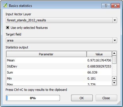
As you can see, the total sum of the stands‘ areas is 66.04 ha.
Note that the area of the missing forest stands is only about 7 ha.
In the same way, you can calculate that the total volume for these stands is
8908 m3/ha and the total number of stems is 179594 stems.
Using the information from the forest stands, instead of directly using that from the sample plots, gives the following average estimates:
184.9 m3/haand2719 stems/ha.
Save your QGIS project, forest_inventory.qgs.
14.7.4. In Conclusion
You managed to calculate forest estimates for the whole forest using the information from your systematic sample plots, first without considering the forest characteristics and also using the interpretation of the aerial image into forest stands. And you also got some valuable information about the particular stands, which could be used to plan the management of the forest in the coming years.
14.7.5. What’s Next?
In the following lesson, you will first create a hillshade background from a LiDAR dataset which you will use to prepare a map presentation with the forest results you just calculated.