Svarbu
Vertimas yra bendruomenės pastangos, prie kurių jūs galite prisijungti. Šis puslapis šiuo metu išverstas 100.00%.
11.2. Sluoksnių kūrimas
Sluoksnius galima kurti įvairiais būdais, pavyzdžiui:
kurti tuščią sluoksnį nuo nulio
kurti sluoksnį pagal esamus sluoksnius
kurti sluoksnį iš iškarpinės
sluoksniai kaip SQL-tipo užklausos rezultatas iš vieno ar daugiau sluoksnių (virtualūs sluoksniai)
QGIS taipogi teikia įrankius importavimui/eksportavimui iš/į skirtingus formatus.
11.2.1. Naujų vektorinių sluoksnių kūrimas
QGIS leidžia jums kurti naujus sluoksnius skirtingais formatais. Jis teikia įrankius, leidžiančius kurti GeoPackage, Shapefile, SpatiaLite, GPX formatais ir Laikinus juodraštinius sluoksnius (dar žinomus kaip atminties sluoksniai). Naujo GRASS sluoksnio kūrimas palaikomas iš GRASS priedo.
11.2.1.1. Naujo GeoPackage sluoksnio kūrimas
Kad sukurtumėte naują GeoPackage sluoksnį, spauskite mygtuką  , kurį rasite meniu arba įrankinėje Duomenų šaltinių tvarkyklė. Taipogi galite sukurti naują GeoPackage sluoksnį Naršyklės skydelyje parinktę Kurti duomenų bazę ir sluoksnį…. Bus parodytas dialogas Naujas GeoPackage sluoksnis, kaip matome paveiksle Fig. 11.26.
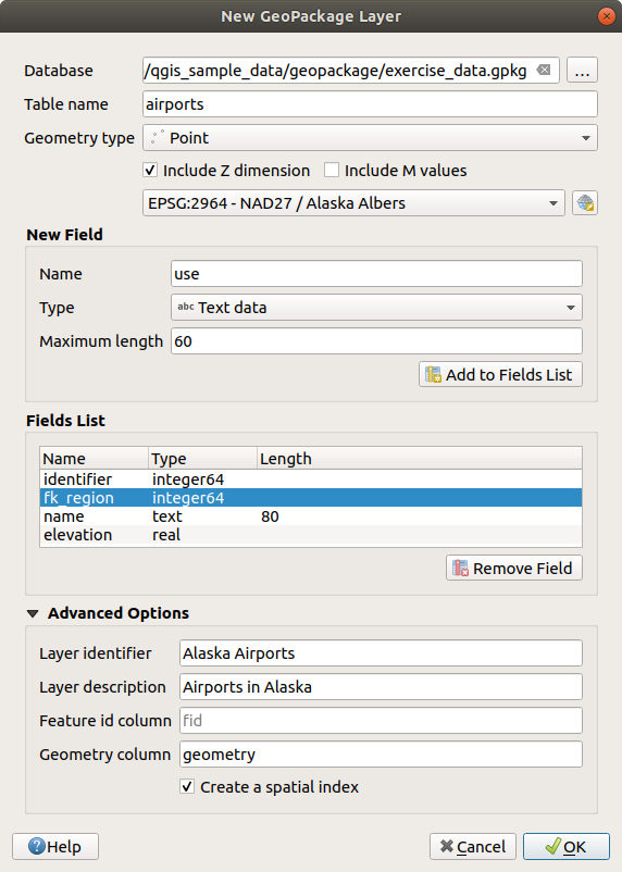
Fig. 11.26 Naujo GeoPackage sluoksnio kūrimo dialogas
Pirmas žingsnis yra nurodyti duomenų bazės failo vietą. Tai galima padaryti paspaudus mygtuką …, kuris yra lauko Duombazė dešinėje ir parinkus esamą GeoPackage failą arba sukūrus naują. QGIS automatiškai pridės reikiamą plėtinį prie jūsų nurodyto pavadinimo.
Nurodykite naujo sluoksnio / lentelės pavadinimą (Lentelės pavadinimas)
Apibrėžkite Geometrijos tipą. Jei tai nėra sluoksnis be geometrijos, jūs galite nurodyti, ar jame turi reikia Įtraukti Z matmenį ir/ar Įtraukti M reikšmes.
Naudodami mygtuką
 nurodykite koordinačių atskaitos sistemą
Norėdami pridėti laukus į jūsų kuriamą sluoksnį:
Įveskite lauko Pavadinimą
Parinkite duomenų Tipą. Palaikomi tipai yra Tekstiniai duomenys, Sveiki skaičiai (integer ir integer64), Dešimtainiai skaičiai, Datos ir Datos su lauku, Dvejetainiai (BLOB) ir Loginiai.
Priklausomai nuo parinkto duomenų formato, įveskite reikšmių Maksimalų ilgį.
Spauskite mygtuką
 Pridėti į laukų sąrašą
Kartokite aukščiau pateiktus veiksmus kiekvienam pridedamam laukui
Vėliau galite keisti laukų rikiuotę naudodami mygtukus
 Perkelti aukštyn ir
  Perkelti žemyn
Kai jums jau tinka atributai, spauskite Gerai. QGIS pridės naują sluoksnį į legendą ir jūs galėsite redaguoti jį kaip aprašyta skyriuje Digitizing an existing layer.
Pagal nutylėjimą, kuriant GeoPackage sluoksnį QGIS sukuria Geoobjekto id lauką pavadinimu fid, kuris veikia kaip sluoksnio pirminis raktas. Pavadinimą galima pakeisti. Geometrijos laukas, jei toks yra, vadinamas geometry ir jūs galite pasirinkti Sukurti jam erdvinį indeksą. Šias parinktis rasite tarp Sudėtingesnių parinkčių, kartu su Sluoksnio identifikatoriumi (trumpu žmogui skaitomu sluoksnio pavadinimu) bei Sluoksnio aprašymu.
Tolimesnį GeoPackage sluoksnių tvarkymą galima atlikti su DB tvarkykle.
11.2.1.2. Naujo Shape failų sluoksnio kūrimas
Norėdami sukurti naują ESRI Shape failų formato sluoksnį, spauskite mygtuką  meniu arba per Duomenų šaltinių tvarkyklės įrankinėje. Dialogas Naujas Shape failo sluoksnis bus rodomas kaip parodyta Fig. 11.27.
Nurodykite kelią ir failo pavadinimą naudodami mygtuką …, esantį greta Failo pavadinimas. QGIS automatiškai pridės tinkamą praplėtimą prie jūsų pateikto pavadinimo.
Tada nurodykite duomenų Failo koduotę
Parinkite sluoksnio Geometrijos tipą: Be geometrijos (tai reikš
.DBFformato failą), taškas, multitaškas, linija arba poligonasNurodykite ar geometrija turi turėti papildomus matmenis: Jokių, Z (+ M reikšmės) ar M reikšmės
Naudodami mygtuką
nurodykite koordinačių atskaitos sistemą
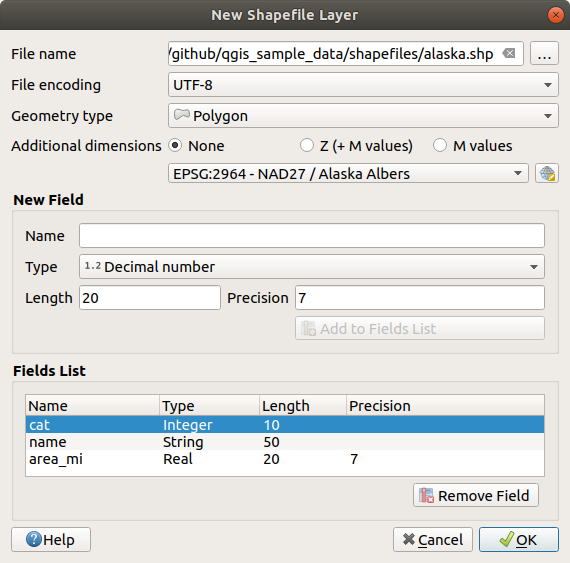
Fig. 11.27 Shape failo sluoksnio kūrimo dialogas
Norėdami pridėti laukus į jūsų kuriamą sluoksnį:
Įveskite lauko Pavadinimą
Parinkite duomenų Tipą. Palaikomi tik Dešimtainių skaičių, Sveikų skaičių, Tekstinių duomenų, Datos ir Loginiai duomenų tipų atributai.
Priklausomai nuo parinkto duomenų formato, įveskite Ilgį ir Tikslumą.
Spauskite mygtuką
Pridėti į laukų sąrašąKartokite aukščiau pateiktus veiksmus kiekvienam pridedamam laukui
Vėliau galite keisti laukų rikiuotę naudodami mygtukus
Perkelti aukštyn ir Perkelti žemynKai jums jau tinka atributai, spauskite Gerai. QGIS pridės naują sluoksnį į legendą ir jūs galėsite redaguoti jį kaip aprašyta skyriuje Digitizing an existing layer.
Pagal nutylėjimą pirmas pridedamas sveiko skaičiaus stulpelis id, bet jį galima išimti.
11.2.1.3. Naujo SpatiaLite sluoksnio kūrimas
Norėdami sukurti naują SpatiaLite sluoksnį, spauskite mygtuką  , kurį rasite meniu arba įrankinėje Duomenų šaltinių tvarkyklė. Jums bus parodytas dialogas Naujas SpatiaLite sluoksnis, kaip pavaizduota Fig. 11.28.
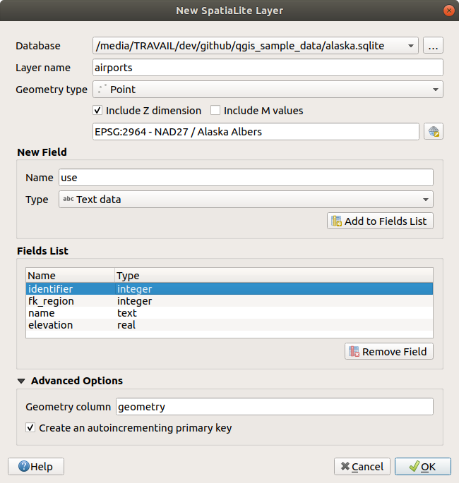
Fig. 11.28 Naujo SpatiaLite sluoksnio kūrimo dialogas
Pirmas žingsnis yra nurodyti duomenų bazės failo vietą. Tai galima padaryti paspaudus mygtuką …, kuris yra lauko Duombazė dešinėje ir parinkus esamą SpatiaLite failą arba sukūrus naują. QGIS automatiškai pridės reikiamą plėtinį prie jūsų nurodyto pavadinimo.
Nurodykite naujo sluoksnio (Sluoksnio pavadinimą)
Apibrėžkite Geometrijos tipą. Jei tai nėra sluoksnis be geometrijos, jūs galite nurodyti, ar jame turi reikia Įtraukti Z matmenį ir/ar Įtraukti M reikšmes.
Naudodami mygtuką
nurodykite koordinačių atskaitos sistemą.
Norėdami pridėti laukus į jūsų kuriamą sluoksnį:
Įveskite lauko Pavadinimą
Parinkite duomenų Tipą. Palaikomi tipai yra Tekstiniai duomenys, Sveiki skaičiai, Dešimtainiai skaičiai, Datos ir Datos su laiku.
Spauskite mygtuką
Pridėti į laukų sąrašąKartokite aukščiau pateiktus veiksmus kiekvienam pridedamam laukui
Vėliau galite keisti laukų rikiuotę naudodami mygtukus
Perkelti aukštyn ir Perkelti žemynKai jums jau tinka atributai, spauskite Gerai. QGIS pridės naują sluoksnį į legendą ir jūs galėsite redaguoti jį kaip aprašyta skyriuje Digitizing an existing layer.
Jei reikia, jūs galite parinkti  Kurti automatiškai didėjantį pirminį raktą skiltyje Sudėtingesnės parinktys. Jūs taipogi galite pervadinti Geometrijos stulpelį (pagal nutylėjimą
 geometry).
Tolimesnį SpatiaLite sluoksnių tvarkymą galima atlikti su DB tvarkykle.
11.2.1.4. Naujo tinklelio sluoksnio kūrimas
Norėdami sukurti naują Tinklelio sluoksnį, spauskite  , kurį rasite meniu arba įrankinėje Duomenų šaltinių tvarkyklė. Pamatysite dialogą Naujas tinklelio sluoksnis tokį, koks rodomas Fig. 11.29.

Fig. 11.29 Naujo tinklelio sluoksnio kūrimo dialogas
Pirmas žingsnis yra nurodyti tinklelio failo vietą. Tai galima padaryti paspaudus mygtuką …, kurį rasite lauko Failo pavadinimas dešinėje, ir parinkus esamą tinklelio failą arba sukūrus naują.
Nurodykite pavadinimą (Sluoksnio pavadinimas), t.y. pavadinimą sluoksnio, kuris rodomas skydelyje Sluoksniai
Parinkite Failo formatą: šiuo metu palaikomi tinklelio failo formatai yra
2DM tinklelio failas (*.2dm),Selafin failas (*.slf)irUGRID (*.nc).Nurodykite duomenų rinkinio Koordinačių atskaitos sistemą
Aukščiau aprašyti žingsniai sukurs tuščią sluoksnį, kuriame jūs vėliau galite skaitmeninti viršūnes ir pridėti jas į grupes. Kaip bebūtų, galima sluoksnį ir inicializuoti su esamu tinklelio sluoksniu, t.y. užpildyti naują sluoksnį viršūnėmis ar plokštumomis iš kito sluoksnio. Norėdami tai padaryti:
Įjunkite parinktį
Inicializuoti tinklelį naudojantparinkite arba Tinklelis iš dabartinio projekto ar Tinklelis iš failo. Parinkto tinklelio failo informacija rodoma patikrinimui.
Pastebėtina, kad į naują sluoksnį perkeliamas tik tinklelio sluoksnio karkasas, duomenų aibės nekopijuojamos.
11.2.1.5. Naujo GPX sluoksnio kūrimas
Norėdami sukurti naują GPX failą:
Parinkite punktą
 , kurį rasite meniu .
Dialoge nurodykite, kur įrašyti naują failą bei koks jo pavadinimas ir spauskite Įrašyti.
Į Sluoksnių skydelį pridedami trys nauji sluoksniai:
taškų sluoksnis vietų (
waypoints) skaitmeninimui su laukais, kuriuose įrašomas pavadinimas, aukštis, komentaras, aprašymas, šaltinis, url ir url pavadinimaslinijų sluoksnis skaitmeninimui sekų vietų, sudarančių planuojamą maršrutą (
routes) su laukais, kuriuose įrašomas pavadinimas, simbolis, numeris, komentaras, aprašymas, šaltinis, url ir url pavadinimasir linijų sluoksnis, kuriame sekamas imtuvo judėjimas laike (
tracks) su laukais, kuriuose įrašomas pavadinimas, simbolis, numeris, komentaras, aprašymas, šaltinis, url ir url pavadinimas.
Dabar jūs galite redaguoti juos visus taip, kaip aprašyta skiltyje Digitizing an existing layer.
11.2.1.6. Naujo laikino juodraštinio sluoksnio kūrimas
Laikini juodraštiniai sluoksniai yra atmintyje laikomi sluoksniai, tai reiškia, kad jie neįrašomi į diską ir bus išmesti, kai QGIS bus uždarytas. Jie gali būti patogūs laikyti geoobjektus, kurie reikalingi tik trumpai, ar kaip tarpiniai sluoksniai tarp veiksmų.
Norėdami sukurti naują Laikiną juodraštinį sluoksnį, parinkite  , kurį rasite meniu arba įrankinėje Duomenų šaltinių tvarkyklė. Pamatysite dialogą Naujas laikinas juodraštinis sluoksnis tokį, koks rodomas Fig. 11.30. Tada:
Nurodykite Sluoksnio pavadinimą
Parinkite Geometrijos tipą. Jūs galite sukurti:
sluoksnį
Be geometrijos, kuris veiks kaip paprasta lentelė,TaškųarMultiTaškųsluoksnį,Linijų/KreiviųarMultiLinijų/MultiKreiviųsluoksnį,Poligonų/KreiviųPoligonųarMultiPoligonų/MultiPaviršiųsluoksnį.
Geometrijos tipams nurodykite duomenų rinkinio matmenis: parinkite, ar reikia Įtraukti Z matmenį ir/ar Įtraukti M reikšmes
Naudodami mygtuką
nurodykite koordinačių atskaitos sistemą.Pridėkite į sluoksnį laukus. Pastebėtina, kad kitaip nei su dauguma kitų formatų, laikiną sluoksnį galima sukurti be jokių laukų. Šis žingsnis neprivalomas.
Įveskite lauko Pavadinimą
Parinkite duomenų Tipą, palaikomi tipai yra: Tekstas, Sveikas skaičius, Dešimtainis skaičius, Loginis, Data, Laikas, Data ir laikas ir Dvejetainis (BLOB).
Priklausomai nuo parinkto duomenų formato, įveskite Ilgį ir Tikslumą
Spauskite mygtuką
Pridėti į laukų sąrašąKartokite aukščiau pateiktus veiksmus visiems pridedamiems laukams
Vėliau galite keisti laukų rikiuotę naudodami mygtukus
Perkelti aukštyn ir Perkelti žemyn
Kai nustatymai bus tinkami, spauskite Gerai. QGIS pridės naują sluoksnį į skydelį Sluoksniai ir jūs galėsite jį redaguoti, kaip aprašyta skiltyje Digitizing an existing layer.
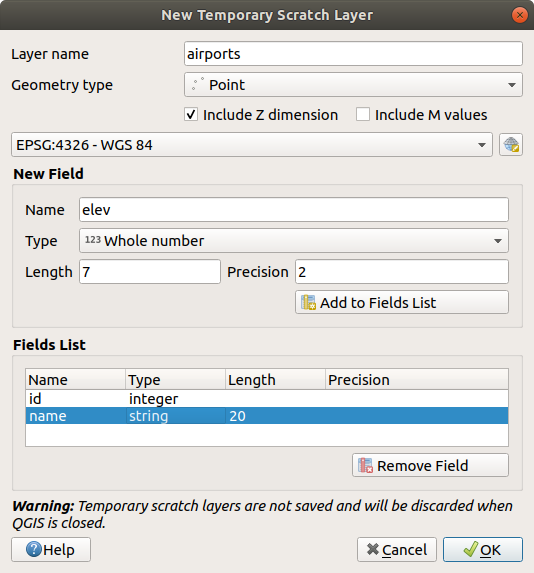
Fig. 11.30 Naujo laikino juodraštinio sluoksnio kūrimo dialogas
Jūs taipogi galite sukurti iš anksto užpildytą laikiną juodraštinį sluoksnį naudojant, pavyzdžiui, iškarpinę (žr. Naujų sluoksnių kūrimas iš iškarpinės) ar kaip Apdorojimo algoritmo rezultatą.
Patarimas
Visam laikui įrašykite laikiną sluoksnį į diską
Kad išvengtumėte duomenų praradimo uždarant projektą su laikinu juodraštiniu sluoksniu, jūs galite įrašyti šiuos sluoksnius į bet kokį QGIS palaikomą formatą:
spauskite greta sluoksnio esantį ženkliuką
 ;
;sluoksnio kontekstiniame meniu parinkite įrašą Padaryti pastoviu;
naudokite kontekstinio meniu punktą ar meniu .
Kiekviena iš šių komandų atidaro dialogą Įrašyti vektorinį sluoksnį kaip, aprašyta skiltyje Naujų sluoksnių kūrimas iš esamų ir įrašytas failas pakeičia laikiną sluoksnį skydelyje Sluoksniai.
11.2.2. Naujų sluoksnių kūrimas iš esamų
Sluoksnius (rastro, vektorinius ir taškų masyvo) galima įrašyti kitu formatu ir/arba perprojektuoti į kitą koordinačių atskaitos sistemą (CRS) naudojant meniu arba paspaudus dešinį pelės mygtuką Sluoksnių skydelyje ir parinkus:
rastro ir taškų masyvo sluoksniams
ar vektoriniams sluoksniams.
Tempkite ir numeskite sluoksnį iš sluoksnių medžio į PostgreSQL įrašą Naršyklės skydelyje. Pastebėtina, kad turite turėti PostgreSQL jungtį Naršyklės skydelyje.
11.2.2.1. Bendri parametrai
Dialogas Įrašyti sluoksnį kaip… rodo kelis parametrus, keičiančius sluoksnio įrašymo elgseną. Tarp bendrų rastro ir vektorių parametrų yra:
Failo pavadinimas: failo vieta diske. Tai gali būti išvesties sluoksnis ar talpykla, kurioje yra sluoksnis (pavyzdžiui duomenų bazės tipo formatai, tokie kaip GeoPackage, SpatiaLite ar Open Document Spreadsheets).
CRS: gali būti pakeista, jei reikia perprojektuoti duomenis
Apimtis: apriboja eksportuojamos įvesties apimtį naudojant valdiklį extent_selector
Pridėti įrašytą failą į žemėlapį: kad naujas sluoksnis būtų pridėtas į drobę
Visgi kai kurie parametrai priklauso nuo konkretaus formato:
11.2.2.2. Rastro parametrai
Priklausomai nuo eksportuojamo formato, kai kurios iš šių parinkčių gali būti negalimos:
Išvesties režimas (jis gali būti pradiniai duomenys ar nubraižytas vaizdas)
Formatas: eksportuoja į bet kokį rastro formatą, kurį moka rašyti GDAL, pavyzdžiui GeoTiff, GeoPackage, MBTiles, Geospatial PDF, SAGA GIS Binary Grid, Intergraph Raster, ESRI .hdr Labelled…
Raiška
Kūrimo parinktys: kuriant failus naudoti sudėtingesnes parinktis (failo suspaudimą, bloko dydį, spalvometriją…), arba iš nuo išvesties formato priklausančių iš anksto apibrėžtų kūrimo profilių, arba rankomis nustatant kiekvieną parametrą.
Piramidžių kūrimas
VRT kaladėlės, jei pasirinkote
Kurti VRTNėra duomenų reikšmės
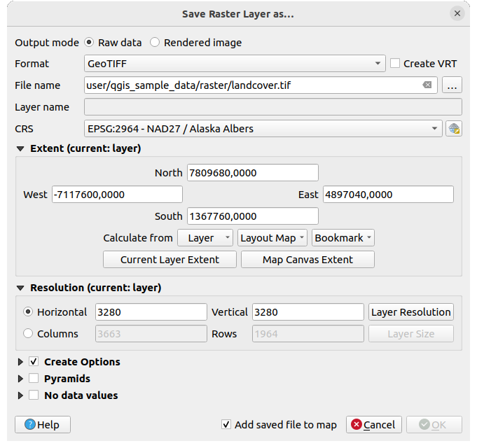
Fig. 11.31 Įrašymas kaip naujo rastro sluoksnio
11.2.2.3. Vektorių parametrai
Priklausomai nuo eksportuojamo formato, gali būti galimos kai kurios iš šių parinkčių:
Formatas: eksportuoja į bet kokį vektorinį formatą, kurį moka rašyti GDAL, tai gali būti GeoPackage, GML, ESRI Shapefile, AutoCAD DXF, ESRI FileGDB, Mapinfo TAB ar MIF, SpatiaLite, CSV, KML, ODS, …
Sluoksnio pavadinimas: galimas, kai Failo pavadinimas nurodo konteinerio tipo formatą, šis laukas nurodys išvesties sluoksnį.
Koduotė
Įrašyti tik parinktus geoobjektus
Parinkite eksportuojamus laukus ir jų eksportavimo parinktis: teikia būda eksportuoti laukus savais pavadinimais ir formų valdiklio nustatymai:
Ties stulpeliu Pavadinimas parinkite eilutes, kurių laukus reikia palikti išvesties sluoksnyje arba spauskite mygtuką Parinkti viską ar Neparinkti nieko
Perjunkite parinktį Naudoti pseudonimus eksportuojamiems pavadinimams, kad užpildytumėte Eksportuojamas pavadinimas stulpelį atitinkamo lauko pseudonimais ar nustatytumėte pradinį lauko pavadinimą. Du kartus paspaudus celę taipogi bus galima redaguoti pavadinimą.
Priklausomai nuo to, ar naudojami atributai iš savų valdiklių, jūs galite Pakeisti visas pradines laukų reikšmes rodomomis reikšmėmis. Pavyzdžiui, jei laukui taikomas valdiklis
reikšmių žemėlapis, išvesties sluoksnyje bus aprašymo reikšmės, o ne pradinės reikšmės. Pakeitimą galima atlikti konkretiems laukams stulpelyje Keisti rodomomis reikšmėmis.
Išlaikyti sluoksnio metaduomenis: užtikrina, kad visi šaltinio sluoksnyje esantys sluoksnio metaduomenys bus nukopijuoti ir įrašyti:
naujai sukurtame sluoksnyje, jei išvestis yra GeoPackage formato
kitiems formatams -
.qmdfaile greta išvesties sluoksnio. Pastebėtina, kad failais paremti formatai, kurie palaiko daugiau nei vieną duomenų rinkinį (pvz. SpatiaLite, DXF,…), gali turėti netikėtą elgseną.
Simbologijos eksportas: galima naudoti pagrinde DXF eksportui ir visiems failų formatams, kurie valdo OGR geoobjektų stilius (žr. pastabą žemiau) kaip DXF, KML, tab failų formatus:
Be simbologijos: numatytasis aplikacijos stilius, kuris skaito duomenis
Geoobjektų simbologija: įrašyti stilių su OGR geoobjektų stiliais (žr. pastabą žemiau)
Simbolių sluoksnio simbologija: įrašyti su OGR geoobjektų stiliais (žr. pastabą žemiau), bet eksportuoti tas pačias geometrijas kelis kartus, jei naudojamas daugiau nei vienas simbologijos sluoksnis
Mastelio reikšmę galima taikyti paskutinėms parinktims
Pastaba
OGR geoobjektų stilius yra būdas saugoti stilių tiesiai duomenyse kaip paslėptą atributą. Tik kai kurie formatai palaiko tokį informacijos tipą. Tokie failų formatai yra KML, DXF ir TAB. Sudėtingesnes detales rasite OGR geoobjektų stilių specifikacijos dokumente.
Geometrija: jūs galite konfigūruoti išvesties sluoksnio geometrijos galimybes
geometrijos tipas: palieka pradinę geoobjektų geometriją, jei parinkta Automatinis, kitais atvejais išmeta ar permuša jį bet kuriuo tipu. Jūs galite pridėti tuščią geometrijos stulpelį į atributų lentelę ir išimti erdvinio sluoksnio geometrijos stulpelį.
Priversti multi-tipą: priverčia milti-geometrijų geoobjektų kūrimą šiame sluoksnyje.
Įtraukti z-matmenis geometrijose.
Patarimas
Sluoksnio geometrijos tipo permušimas leidžia atlikti tokius dalykus kaip įrašyti lentelę be geometrijos (pvz. .csv failą) į shape failą SU bet kokiu geometrijos tipu (taškas, linija, poligonas), kad vėliau būtų galima rankiniu būdu į įrašus pridėti geometrijas naudojant įrankį  Pridėti dalį.
Duomenų šaltinių parinktys, Sluoksnio parinktys ar Savo parinktys, kurios leidžia jums konfigūruoti sudėtingesnius parametrus priklausomai nuo išvesties formato. Kai kurios aprašytos Exploring Data Formats and Fields, bet pilną informaciją rasite GDAL tvarkyklės dokumentacijoje. Kiekvienas failo formatas turi savo parametrus, pavyzdžiui
GeoJSONformato atveju skaitykite GDAL GeoJSON dokumentaciją.
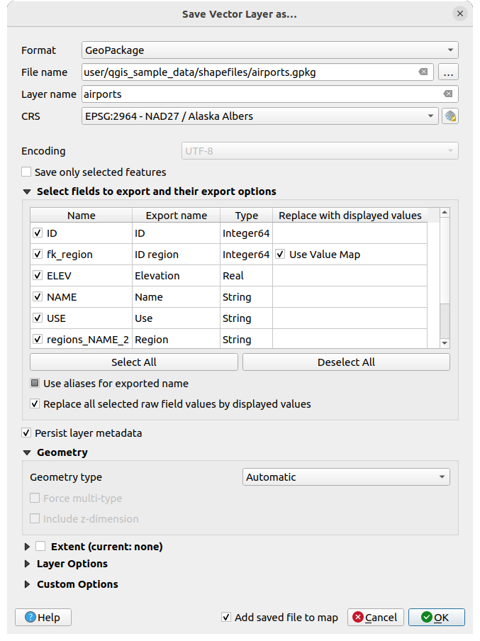
Fig. 11.32 Įrašymas kaip naujo vektorinio sluoksnio
Įrašant vektorinį sluoksnį į esamą failą, priklausomai nuo išvesties failo formato galimybių (Geopackage, SpatiaLite, FileGDB…), naudotojas gali pasirinkti ar:
perrašyti visą failą
perrašyti tik paskirties sluoksnį (galima konfigūruoti sluoksnio pavadinimą)
pridėti geoobjektus į esamą paskirties sluoksnį
pridėti geoobjektus, pridėti naujus laukus, jei tokių yra.
Formatams, tokiems kaip ESRI Shapefile, MapInfo .tab, galima taipogi papildyti geoobjektus.
11.2.2.4. Taškų masyvo parametrai
Panašiai kaip rastrų ir vektorių sluoksniams, taškų masyvų sluoksnius galima įrašyti skirtingais formatais ir/arba perprojektuoti į kitą koordinačių atskaitos sistemą (CRS). Tai leidžia jums eksportuoti taškų masyvų sluoksnius į vektorių ar taškų masyvų formatus. Šiuo metu palaikomi formatai yra: Laikinas juodraštinis (atminties sluoksnis), GeoPackage, ESRI Shapefile, DXF ir LAS/LAZ taškų masyvas. Be bendrų aukščiau išvardintų parametrų, eksportuojant į taškų masyvų sluoksnius, galima naudoti šias parinktis:
Filtruoti pagal poligonų sluoksnį: leidžia jums filtruoti taškų masyvo duomenis pagal poligonų sluoksnį.
Aukščio diapazonas: leidžia filtruoti taškų masyvo duomenis pagal nurodytą Z diapazoną.
Riboti taškų skaičių: suteikia parinktį riboti iš taškų masyvo sluoksnio eksportuojamų taškų skaičių.
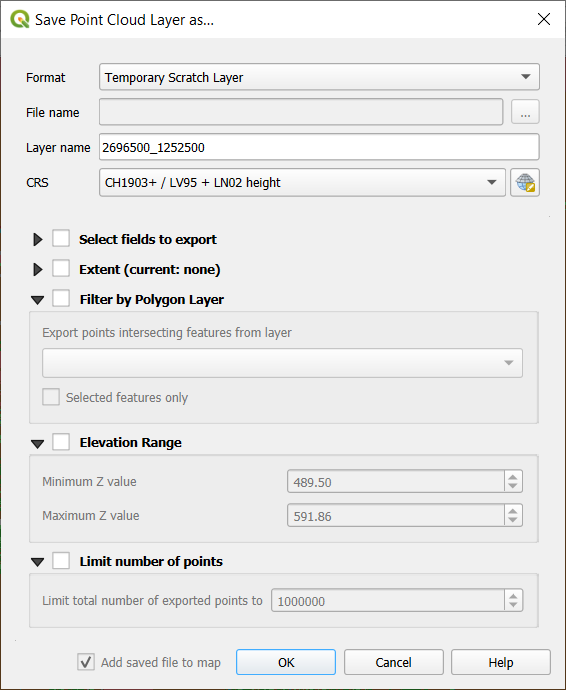
Fig. 11.33 Taškų masyvo sluoksnio įrašymas kaip naujo sluoksnio
11.2.3. Naujų DXF failų kūrimas
Be dialogo Įrašyti kaip…, kuris teikia parinktis eksportuoti vieną sluoksnį į kitą formatą, įskaitant ir *.DXF, QGIS teikia kitą įrankį, leidžiantį eksportuoti kelis sluoksnius kaip vieną DXF sluoksnį. Jį rasite per meniu .
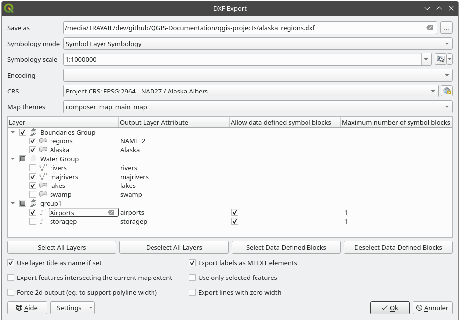
Fig. 11.34 Projekto eksportavimo į DXF dialogas
DXF eksporto dialoge:
Nurodykite paskirties failą.
Parinkite simbologijos režimą ir mastelį (žr. pastabą apie OGR geoobjektų stilius), jei jis taikomas.
Parinkite duomenų Koduotę.
Parinkite taikomą CRS: parinkti sluoksniai bus perprojektuoti į nurodytą CRS.
Parinkite sluoksnius, kuriuos reikia įtraukti į DXF failus, arba juos pažymėdami lentelės valdiklyje, arba automatiškai juos parinkdami iš esamos žemėlapio temos. Mygtukai Parinkti viską ir Neparinkti nieko gali padėti jums greitai nurodyti eksportuojamus duomenis.
Kiekvienam sluoksniui jūs galite:
Permušti išvesties sluoksnio pavadinimą nekeičiant pradinio projekto sluoksnio. Tam spauskite Sluoksnio pavadinimą dialoge ir įrašykite išvestyje naudotiną pavadinimą.
Išvesties sluoksnio atributai: Parinkite ar eksportuoti visus geoobjektus viename DXF sluoksnyje, ar remtis lauku, kurio reikšmės būtų naudojamos atskirti geoobjektus į atskirus sluoksnius DXF išvestyje. Paskutiniu atveju kiekvienas sluoksnis bus pavadintas pagal atitinkamo lauko reikšmę.
Leisti pagal duomenis apibrėžiamus simbolių blokus:
Maksimalus simbolių blokų skaičius: kuria simbolių blokus iki nurodytos ribos, pradedant tais, kurie turi didžiausią nuorodų skaičių. Kiti simboliai įrašomi tokie, kokie jie yra.
-1reiškia, kad apribojimo nėra.
Pasirinktinai dar galite:
 Naudoti sluoksnio antraštę, kaip pavadinimą, jei ji nurodyta, vietoje sluoksnio pavadinimo: antraštė imama iš metaduomenų arba serverio sluoksnio savybių;
- Eksportuoti geoobjektus, kertančius dabartinę žemėlapio apimtį;
- Priverstinai kurti 2d išvestį (pvz. palaikyti polilinijos plotį);
- Eksportuoti užrašus kaip MTEXT elementus ar TEXT elementus;
- Naudoti tik parinktus geoobjektus;
- Eksportuoti linijas su nuliniu pločiu: jungus visos linijos eksportuojamos su minimaliu pločiu
0(plauko). Tai padeda linijas faile laikyti minimaliomis nepriklausomai nuo mastelio ir gali būti patogu darant tolimesnį CAD-redagavimą su eksportuotu dxf, ypač jei žemėlapyje yra daug vienas šalia kito esančių geoobjektų.
Pastaba
Išvesties sluoksnio pavadinimo apibrėžimo prioritetas yra toks:
Reikšmė lauke Išvesties sluoksnio atributas
Permuštas pavadinimas stulpelyje Sluoksnis
Parinktis Naudoti sluoksnio antraštę kaip pavadinimą, jei nurodyta
Sluoksnio pavadinimas
Dabartinius nustatymus, apibrėžtus dialoge DXF eksportas, galima įrašyta į XML failą ir vėliau iš naujo panaudoti kitose sesijose. Tam Nustatymų mygtukas turi dvi parinktis: Įkelti nustatymus iš failo… ir Įrašyti nustatymus į failą….
11.2.4. Naujų sluoksnių kūrimas iš iškarpinės
Iškarpinėje esančius geoobjektus galima įkelti į naują sluoksnį. Norėdami tai padaryti, parinkite kelis geoobjektus, nukopijuokite juos į iškarpinę ir tada įkelkite juos į naują sluoksnį naudodami meniu ir ten parinkdami:
Naujas vektorinis sluoksnis…: pasirodys dialogas Įrašyti vektorinį sluoksnį kaip… (žr. Naujų sluoksnių kūrimas iš esamų parametrų sąrašui)
arba Laikinas juodraštinis sluoksnis…: jums reikės nurodyti sluoksnio pavadinimą
Sukuriamas (ir pridedamas į žemėlapio drobę) naujas sluoksnis, užpildytas parinktais geoobjektais ir jų atributais.
Pastaba
Kurti sluoksnius iš iškarpinės galima tiek geoobjektus parinkus ir nukopijavus su QGIS, tiek ir su kitomis aplikacijomis, jei jų geometrijos apibrėžiamos naudojant gerai žinomą tekstą (WKT).
11.2.5. SQL užklausų sluoksnių kūrimas
Be viso sluoksnio įkėlimo į projektą ar naujų sluoksnių kūrimo nuo nulio ar įkeltų geoobjektų, jūs taipogi galite įkelti sluoksnius, kurie sukurti iš kito(ų) sluoksnio(ių). Jie yra rezultatas daugiau ar mažiau sudėtingo filtro, naudojančio SQL kalbą, pritaikyto įrašytiems sluoksniams nepriklausomai nuo duomenų tiekėjo ar jų prieinamumo aktyviame projekte. Tai reiškia, kad laikini sluoksniai nesuderinami su šia savybe. Priklausomai nuo tiekėjo, užklausoje galima naudoti vieną arba daugiau sluoksnių. Sukurtas sluoksnis liks nepriklausomas nuo užklausoje panaudoto(ų) sluoksnio(ių), ir jis įkeliamas naudojant greta esančią piktogramą  Filtras.
Ši savybė prieinama:
Naršyklės skydelyje, spauskite dešinį pelės mygtuką ant palaikomų duomenų (paprastas sluoksnis, duomenų bazės jungtis, schema ar lentelė) ir kontekstiniame meniu parinkite Vykdyti SQL….
Sluoksnių skydelyje, parinkite įkeltą sluoksnį, spauskite dešinį pelės mygtuką ir kontekstiniame meniu parinkite Vykdyti SQL….
Tai atvers langą su centriniu teksto įvedimo valdikliu, kur jūs galėsite rašyti SQL užklausas.

Fig. 11.35 SQL užklausų vykdymas SQL vykdymo lange
Dialogo viršuje dialogas teikia įrankinę su rinkinių įrankių, skirtų kurti, saugoti ir keisti jūsų užklausas:
 Atverti užklausas…: užpildo redaktoriaus valdiklį turiniu iš esamo
 .sqlfailo Įrašyti užklausas… ir
  Įrašyti užklausas kaip… padeda jums įrašyti užklausas į
 .sqlfailąUžklausas galima keisti naudojant mygtukus
 Iškirpti,
  Kopijuoti ir
  Įkelti. Taip pat galite
  Atšaukti ar
  Pakartoti jūsų pakeitimus.
 Rasti ir pakeisti įjungia dialogo apačioje valdiklį, kuris leidžia ieškoti konkretaus teksto jūsų SQL kode. Paieška gali atsižvelgti į raidžių dydį, ieškoti dalinio ar pilno žodžio, remtis reguliaria išraiška. Tada galima pereiti per visas rastas eilutes, pakeičiant jas po vieną arba visas kartu.
Naudokite
 Išvalyti SQL redaktorių, jei norite ištrinti visą tekstą.
Mygtukas
 Istorija atveria dialogą, kuriame yra anksčiau vykdytos užklausos. Daugiau informacijos rasite Užklausų istoriją.
Kaip minėta anksčiau, užklausas galima įrašyti kaip
.sqlfailą diske. Naudojant mygtuką Įrašyti dabartinę užklausą jas taipogi galima įrašyti:
aktyviame Naudotojo profilyje, susijusiame
QGIS3.inifaile, taip jis būtų prieinamas kituose projektuosekaip Dabartinio projekto dalį.
Paspaudus įrašą įrašytų užklausų iškrentančiame meniu įterpia tą užklausą į tuo metu rašomą išraišką. Įrašytą įrašą taipogi galima ištrinti per iškrentantį meniu.
11.2.5.1. Užklausų vykdymas ir įkėlimas kaip sluoksnio
Centrinėje Vykdyti SQL dialogo dalyje jūs kuriate jūsų užklausą naudodami SQL sintaksę, kurią palaiko atitinkamas tiekėjas (t.y., OGR, GeoPackage, PostgreSQL).
Pagal nutylėjimą, jei atverta iš sluoksnio įrašo, pateikiama pavyzdinė SQL užklausa. Iš kontekstinio meniu galima naudoti redagavimo įrankius parinkti, iškirpti, kopijuoti, įkelti, atšaukti ir pakartoti.
Patarimas
Jūsų duomenų aibei tinkamos SQL sintaksės paieška
Kad rastumėte jūsų duomenų aibei tinkamą SQL dialektą, spauskite mygtuką …, esantį greta apatinėje dialogo dalyje esančios parinkties Poaibio filtras.
Kai viskas paruošta, spauskite po teksto valdikliu esantį mygtuką Vykdyti, kad vykdytumėte užklausą. Galima pažymėti dalį SQL ir vykdyti tik tą dalį spaudžiant Ctrl+R arba spaudžiant mygtuką Vykdyti pažymėjimą. Norėdami nutraukti vykdymą spauskite mygtuką Stabdyti.
Po sėkmingo užklausos vykdymo dialogo apačioje bus rodoma lentelė su grąžintais geoobjektais. Jūs galite parinkti konkrečias rezultatų rinkinio celes. Naudokite klavišų kombinaciją Ctrl+C, kad nukopijuotumėte parinktas celes į iškarpinę. Nukopijuoti duomenys pasiekiami kaip formatuota lentelė. Tai leidžia jums įkelti duomenis į kitas aplikacijas, tokias kaip skaičiuokles, kur jos matysis kaip lentelė.
Grąžintą lentelę galima įkelti į QGIS išplečiant grupę Įkelti kaip naują sluoksnį ir sukonfigūravus parametrus (jie priklauso nuo sluoksnio tiekėjo):
Stulpelis(iai) su unikaliomis reikšmėmis duomenų pirminio rakto nurodymui,
Geometrijos stulpelis: įjunkite varnelę, kad įkeltumėte sluoksnį kaip erdvinį, ir nurodykite geometrijos lauko pavadinimą
Poaibio filtras: leidžia filtruoti rezultatus naudojant
WHEREsąlygą. Ją galima rašyti teksto lauke arba sukurti naudojant Užklausos kūrėją po to, kai paspaudžiate …. Įsitikinkite, kad naudojate laukus, kurie yra SQL sluoksnyje.Vengti parinkti pagal geoobjekto ID
Sluoksnio pavadinimas projekte
Bet kuriuo metu Sluoksnių skydelyje jūs galite pakeisti išvesties sluoksnį spausdami dešinį pelės mygtuką ir parinkdami Keisti SQL išraišką…. Atidaromas dialogas Keisti SQL, kuriame įrašoma taikoma užklausa, kurią jūs galite keisti. Kai viskas paruošta, spauskite Atnaujinti sluoksnį ir sluoksnis bus pakeistas.
11.2.5.2. Užklausų istoriją
Užklausų istorijos dialogas rodo visas anksčiau vykdytas užklausas, išrikiuotas pagal datą ir duomenų tiekėjo tipą. Jį galima pasiekti per meniu Užklausų istorija… arba paspaudus mygtuką Istorija dialoge Vykdyti SQL.

Fig. 11.36 Vykdytų SQL užklausų istorija
Dialogo viršuje yra paieškos eilutė, kurią galima naudoti užklausų filtravimui. Paieška vykdoma visuose užklausų istorijoje rodomų užklausų tekstuose. Jei dialogas atidaromas iš dialogo Vykdyti SQL, prieš paieškos lauką pridedama Vykdyti SQL įrankinė.
Žemiau sutraukiami ir išrikiuoti datų įrašai rodo atitinkamas jų užklausas. Kiekviena užklausa identifikuojama jos SQL komanda, o išskleidus, parodo:
Jungtį: šaltinį duomenų, kuriais remiasi užklausa
Eilučių skaičių: grąžintų geoobjektų skaičių
Vykdymo laiką
Užveskite pelę virš įrašo ir iššokančioje žymoje bus parodyta pilna užklausa. Analogiškai, pažymėjus įrašą ji bus parodyta apatinėje dialogo dalyje. Jūs galite sąveikauti su tekstu, kopijuoti jį visą ar tik dalį.
Du kartus paspauskite SQL komandos įrašą - bus atidarytas dialogas Vykdyti SQL su užpildyta paspausta užklausa. Bet kokia rašoma užklausa bus perrašyta. Spauskite dešinį pelės mygtuką ant SQL komandos, ir jūs galėsite:
Įkelti SQL komandą…, įkelia paskirties komandą į dialogą Vykdyti SQL, pakeičiant bet kokią ten esančią užklausą. Tai tas pats, kas du kartus paspausti įrašą.
Kopijuoti SQL komandą ir įkelti kur tik norite.
11.2.6. Virtualių sluoksnių kūrimas
Virtualus sluoksnis yra ypatinga vektorinių sluoksnių rūšis. Jis leidžia jums apibrėžti sluoksnį kaip SQL užklausos rezultatą naudojant bet kokį skaičių vektorinių sluoksnių, kuriuos gali atverti QGIS. Virtualūs sluoksniai patys duomenų neturi ir į juos galima žiūrėti kaip į vaizdus.
Kad sukurtumėte virtualų sluoksnį, atverkite virtualaus sluoksnio kūrimo dialogą:
parinkdami įrašą
 Pridėti/keisti virtualų sluoksnį meniu ;
įjungdami kortelę
Pridėti virtualų sluoksnį dialoge Duomenų šaltinių tvarkyklė;ar naudodami DB tvarkyklės dialogo medį.
Dialogas leidžia jums nurodyti Sluoksnio pavadinimą ir SQL Užklausą. Užklausa gali naudoti įkeltų vektorinių sluoksnių pavadinimus (ar id) kaip lenteles ir jų laukų pavadinimus kaip stulpelius.
Pavyzdžiui, jei turite sluoksnį, pavadintą airports, jūs galite sukurti naują virtualų sluoksnį vardu public_airports su tokia SQL užklausa:
SELECT *
FROM airports
WHERE USE = "Civilian/Public"
SQL užklausa bus įvykdyta nepriklausomai nuo airports sluoksnio tiekėjo, net jei šis tiekėjas tiesiogiai nepalaiko SQL užklausų.
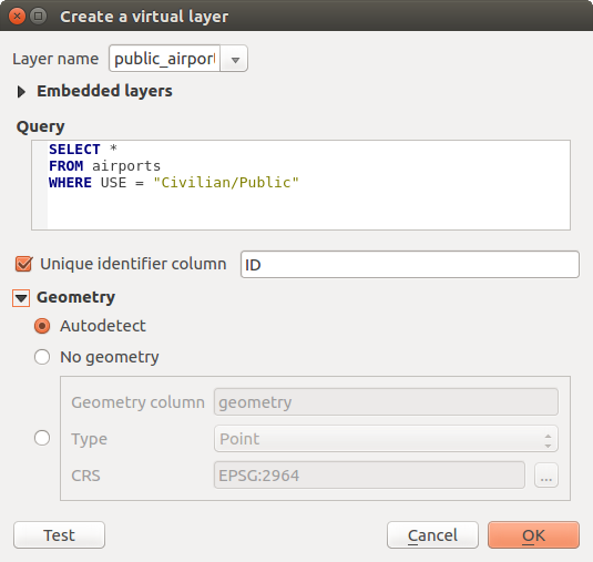
Fig. 11.37 Virtualių sluoksnių kūrimo dialogas
Taipogi galima kurti ir jungtis bei sudėtingas užklausas. Pavyzdžiui jungti oro uostus su šalių informacija:
SELECT airports.*, country.population
FROM airports
JOIN country
ON airports.country = country.name
Pastaba
Virtualius sluoksnius taipogi galima kurti naudojant DB Manager Plugin SQL langą.
11.2.6.1. Įtraukti sluoksniai naudojimui užklausose
Be vektorinių sluoksnių, esančių žemėlapio drobėje, naudotojas gali pridėti sluoksnius į Įtrauktų sluoksnių sąrašą, kurį galima naudoti užklausose be poreikio juos rodyti žemėlapio drobėje ar sluoksnių skydelyje.
Kad įtrauktumėte sluoksnį, spauskite Pridėti ir pateikite Vietinį pavadinimą, Tiekėją, Koduotę ir kelią iki Šaltinio.
Mygtukas Importuoti leidžia pridėti sluoksnius žemėlapio drobės sluoksnius į įtraukiamų sluoksnių sąrašą. Šiuos sluoksnius tada galima išimti iš sluoksnių skydelio nesugadinant jau esamų užklausų.
11.2.6.2. Palaikoma užklausų kalba
Vykdymui naudojami SQLite ir SpatiaLite.
Tai reiškia, kad jūs galite naudoti visą SQL, kurį supranta jūsų vietinė SQLite.
Virtualaus sluoksnio užklausoje galima naudot ir SQLite bei SpatiaLite erdvines funkcijas. Pavyzdžiui kurti taškų sluoksnį iš sluoksnio, kuriame yra tik atributai, galima užklausa, panašia į šią:
SELECT id, MakePoint(x, y, 4326) as geometry
FROM coordinates
QGIS išraiškų funkcijas taipogi galima naudoti virtualių sluoksnių užklausose.
Jei norite naudoti sluoksnio geometrijos stulpelį, naudokite pavadinimą geometry.
Priešingai nei grynose SQL užklausose, virtualių sluoksnių užklausose visiems stulpeliams privalo būti nurodyti pavadinimai. Nepamirškite naudoti raktinio žodžio as nurodant pavadinimus stulpeliams, jei jie yra skaičiavimo ar funkcijų kvietimo rezultatai.
11.2.6.3. Greitaveikos problemos
Su numatytais parametrais virtualaus sluoksnio variklis bandys aptikti užklausos stulpelių tipus, įskaitant ir geometrijos lauko tipą, jei toks laukas yra.
Tai daroma kur įmanoma tiriant pačią užklausą arba, kaip kraštutinę priemonę, ištraukiant pirmą užklausos rezultato įrašą (LIMIT 1). Pirmo įrašo ištraukimas tik tam, kad būtų sukurtas sluoksnis, kartais gali būti nepageidaujama dėl greitaveikos.
Sukūrimo dialogo parametrai:
Unikalaus identifikatoriaus stulpelis: nurodo užklausos lauką, kuris reprezentuoja unikalias reikšmes, kurias QGIS gali naudoti kaip įrašų identifikatorius. Pagal nutylėjimą naudojama automatiškai didėjanti sveiko skaičiaus reikšmė. Unikalaus identifikatoriaus stulpelio nurodymas pagreitina įrašų parinkimą pagal id.
Be geometrijos: priverčia virtualų sluoksnį ignoruoti geometrijos lauką. Bus gautas tik atributų sluoksnis.
Geometrijos Stulpelis: nurodo geometrijos stulpelio pavadinimą.
Geometrijos Tipas: nurodo geometrijos tipą.
Geometrijos CRS: nurodo virtualaus sluoksnio koordinačių atskaitos sistemą.
11.2.6.4. Specialūs komentarai
Virtualaus sluoksnio variklis bando nustatyti kiekvieno užklausos stulpelio tipą. Jei jam tai nepavyksta, ištraukiamas pirmas užklausos grąžinamas įrašas, kad iš jo būtų galima nustatyti stulpelių tipus.
Konkretaus stulpelio tipą galima nurodyti tiesiogiai užklausoje, naudojant specialiai parašytus komentarus.
Sintaksė yra tokia: /*:tipas*/. Komentaras turi būti parašytas iš karto po stulpelio pavadinimo. tipas gali būti int sveikiems skaičiams, real slankaus kablelio skaičiams arba text.
Pavyzdžiui:
SELECT id+1 as nid /*:int*/
FROM table
Geometrijos stulpelio tipą ir koordinačių atskaitos sistemą galima nurodyti naudojant specialius komentarus su tokia sintakse /*:gtipas:srid*/, kur gtipas yra geometrijos tipas (point, linestring, polygon, multipoint, multilinestring arba multipolygon), o srid - sveikas skaičius - koordinačių atskaitos sistemos EPSG kodas.
11.2.6.5. Indeksų naudojimas
Kai sluoksnis prašomas per virtualų sluoksnį, šaltinio sluoksnio indeksai bus naudojami tokiais būdais:
jei predikatas
=naudojamas su sluoksnio pirminiu raktu, atitinkamo duomenų tiekėjo bus paprašyti konkretaus id (FilterFid)bet kokiems kitiems predikatams (
>,<=,!=ir pan.) arba naudojant ne su pirminio rakto stulpeliu, iš išraiškos sukurta užklausa bus naudojama prašant atitinkamo vektorinių duomenų tiekėjo. Tai reiškia, kad indeksus duomenų tiekėjas gali panaudoti, jei jie yra.
Yra speciali sintaksė, skirta valdyti erdvinius predikatus užklausose ir jie inicijuoja erdvinių indeksų naudojimą: kiekviename virtualiame sluoksnyje yra paslėptas stulpelis pavadinimu _search_frame_. Šį stulpelį galima lyginti su apimties stačiakampiu. Pavyzdžiui:
SELECT *
FROM vtab
WHERE _search_frame_=BuildMbr(-2.10,49.38,-1.3,49.99,4326)
Erdviniai dvejetainiai predikatai, tokie kaip ST_Intersects stipriai pagreitinami, kai naudojami kartu su šia erdvinių indeksų sintakse.